pacman::p_load(sf, tmap, tidyverse)Hands-on Exercise 8a
21 Choropleth Mapping with R
21.2 Getting Started
21.3 Importing Data into R
mpsz <- st_read(dsn = "Data/Master Plan 2014 Subzone Boundary (Web) (SHP)",
                layer = "MP14_SUBZONE_WEB_PL")
Reading layer `MP14_SUBZONE_WEB_PL' from data source
`C:\edwardbyl00\ISSS608-VAA\Hands-on_EX\Hands-on_EX08\Data\Master Plan 2014 Subzone Boundary (Web) (SHP)'
using driver `ESRI Shapefile'
Simple feature collection with 323 features and 15 fields
Geometry type: MULTIPOLYGON
Dimension: XY
Bounding box: xmin: 2667.538 ymin: 15748.72 xmax: 56396.44 ymax: 50256.33
Projected CRS: SVY21mpszSimple feature collection with 323 features and 15 fields
Geometry type: MULTIPOLYGON
Dimension: XY
Bounding box: xmin: 2667.538 ymin: 15748.72 xmax: 56396.44 ymax: 50256.33
Projected CRS: SVY21
First 10 features:
OBJECTID SUBZONE_NO SUBZONE_N SUBZONE_C CA_IND PLN_AREA_N
1 1 1 MARINA SOUTH MSSZ01 Y MARINA SOUTH
2 2 1 PEARL'S HILL OTSZ01 Y OUTRAM
3 3 3 BOAT QUAY SRSZ03 Y SINGAPORE RIVER
4 4 8 HENDERSON HILL BMSZ08 N BUKIT MERAH
5 5 3 REDHILL BMSZ03 N BUKIT MERAH
6 6 7 ALEXANDRA HILL BMSZ07 N BUKIT MERAH
7 7 9 BUKIT HO SWEE BMSZ09 N BUKIT MERAH
8 8 2 CLARKE QUAY SRSZ02 Y SINGAPORE RIVER
9 9 13 PASIR PANJANG 1 QTSZ13 N QUEENSTOWN
10 10 7 QUEENSWAY QTSZ07 N QUEENSTOWN
PLN_AREA_C REGION_N REGION_C INC_CRC FMEL_UPD_D X_ADDR
1 MS CENTRAL REGION CR 5ED7EB253F99252E 2014-12-05 31595.84
2 OT CENTRAL REGION CR 8C7149B9EB32EEFC 2014-12-05 28679.06
3 SR CENTRAL REGION CR C35FEFF02B13E0E5 2014-12-05 29654.96
4 BM CENTRAL REGION CR 3775D82C5DDBEFBD 2014-12-05 26782.83
5 BM CENTRAL REGION CR 85D9ABEF0A40678F 2014-12-05 26201.96
6 BM CENTRAL REGION CR 9D286521EF5E3B59 2014-12-05 25358.82
7 BM CENTRAL REGION CR 7839A8577144EFE2 2014-12-05 27680.06
8 SR CENTRAL REGION CR 48661DC0FBA09F7A 2014-12-05 29253.21
9 QT CENTRAL REGION CR 1F721290C421BFAB 2014-12-05 22077.34
10 QT CENTRAL REGION CR 3580D2AFFBEE914C 2014-12-05 24168.31
Y_ADDR SHAPE_Leng SHAPE_Area geometry
1 29220.19 5267.381 1630379.3 MULTIPOLYGON (((31495.56 30...
2 29782.05 3506.107 559816.2 MULTIPOLYGON (((29092.28 30...
3 29974.66 1740.926 160807.5 MULTIPOLYGON (((29932.33 29...
4 29933.77 3313.625 595428.9 MULTIPOLYGON (((27131.28 30...
5 30005.70 2825.594 387429.4 MULTIPOLYGON (((26451.03 30...
6 29991.38 4428.913 1030378.8 MULTIPOLYGON (((25899.7 297...
7 30230.86 3275.312 551732.0 MULTIPOLYGON (((27746.95 30...
8 30222.86 2208.619 290184.7 MULTIPOLYGON (((29351.26 29...
9 29893.78 6571.323 1084792.3 MULTIPOLYGON (((20996.49 30...
10 30104.18 3454.239 631644.3 MULTIPOLYGON (((24472.11 29...21.3.3 Importing Attribute Data into R
Import respopagsex2011to2020.csv file into RStudio and save the file into an R dataframe called popagsex
popdata <- read_csv("Data/respopagesextod2011to2020.csv")21.3.4 Data Preparation
21.3.4.1 Data wrangling
popdata2020 <- popdata %>%
  filter(Time == 2020) %>%
  group_by(PA, SZ, AG) %>%
  summarise(`POP` = sum(`Pop`)) %>%
  ungroup() %>%
  pivot_wider(names_from=AG,
              values_from=POP) %>%
  mutate(YOUNG = rowSums(.[3:6])
         +rowSums(.[12])) %>%
mutate(`ECONOMY ACTIVE` = rowSums(.[7:11])+
rowSums(.[13:15]))%>%
mutate(`AGED`=rowSums(.[16:21])) %>%
mutate(`TOTAL`=rowSums(.[3:21])) %>%
mutate(`DEPENDENCY` = (`YOUNG` + `AGED`)
/`ECONOMY ACTIVE`) %>%
  select(`PA`, `SZ`, `YOUNG`,
       `ECONOMY ACTIVE`, `AGED`,
       `TOTAL`, `DEPENDENCY`)
21.3.4.2 Joining the attribute data and geospatial data
Convert the values in PA and SZ fields to uppercase
popdata2020 <- popdata2020 %>%
  mutate(across(c(PA, SZ), toupper)) %>%
  filter(`ECONOMY ACTIVE` > 0)
mpsz_pop2020 <- left_join(mpsz, popdata2020,
by = c("SUBZONE_N" = "SZ"))write_rds(mpsz_pop2020, "Data/mpszpop2020.rds")21.4 Choropleth Mapping Geospatial Data Using tmap
21.4.1 Plotting a choropleth map quickly by using qtm()
tmap_mode() with “plot” option is used to produce a static map. For interactive mode, “view” option should be used.
fill argument is used to map the attribute (i.e. DEPENDENCY)
tmap_mode("plot")ℹ tmap modes "plot" - "view"
ℹ toggle with `tmap::ttm()`qtm(mpsz_pop2020,
fill = "DEPENDENCY")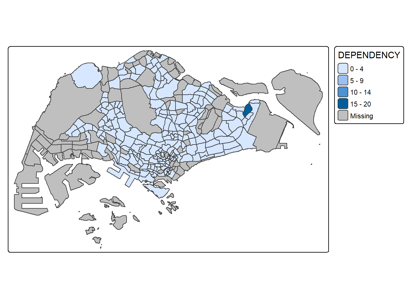
21.4.2 Creating a choropleth map by using tmap’s elements
qtm( )advantages: Able to draw a choropleth map quickly and easily,
Disadvantge of qtm(): It makes aesthetics of individual layers harder to control. To draw a high quality cartographic choropleth map as shown in the figure below, tmap’s drawing elements should be used.
tm_shape(mpsz_pop2020)+
  tm_polygons(fill = "DEPENDENCY",
              fill.scale = tm_scale_intervals(
                style = "quantile",
                n = 5,
                values = "brewer.blues"),
              fill.legend = tm_legend(
                title = "Dependency ratio")) +
  tm_title("Distribution of Dependency Ratio by planning subzone") +
  tm_layout(frame = TRUE) +
  tm_borders(fill_alpha = 0.5) +
  tm_compass(type="8star", size = 2) +
  tm_grid(alpha =0.2) +
  tm_credits("Source: Planning Sub-zone boundary from Urban Redevelopment Authorithy (URA)\n and Population data from Department of Statistics DOS",
             position = c("left", "bottom"))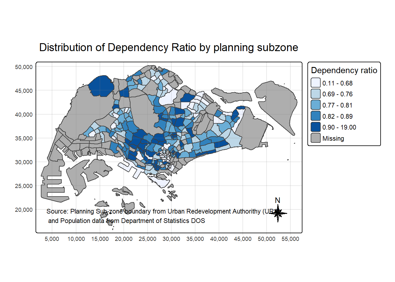
21.4.2.1 Drawing a base map
tm_shape(mpsz_pop2020) +
  tm_polygons()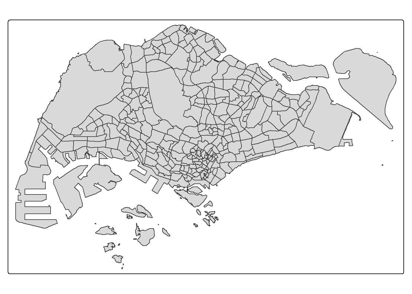
21.4.2.2 Drawing a choropleth map using tm_polygons()
With line border
tm_shape(mpsz_pop2020)+
  tm_polygons("DEPENDENCY")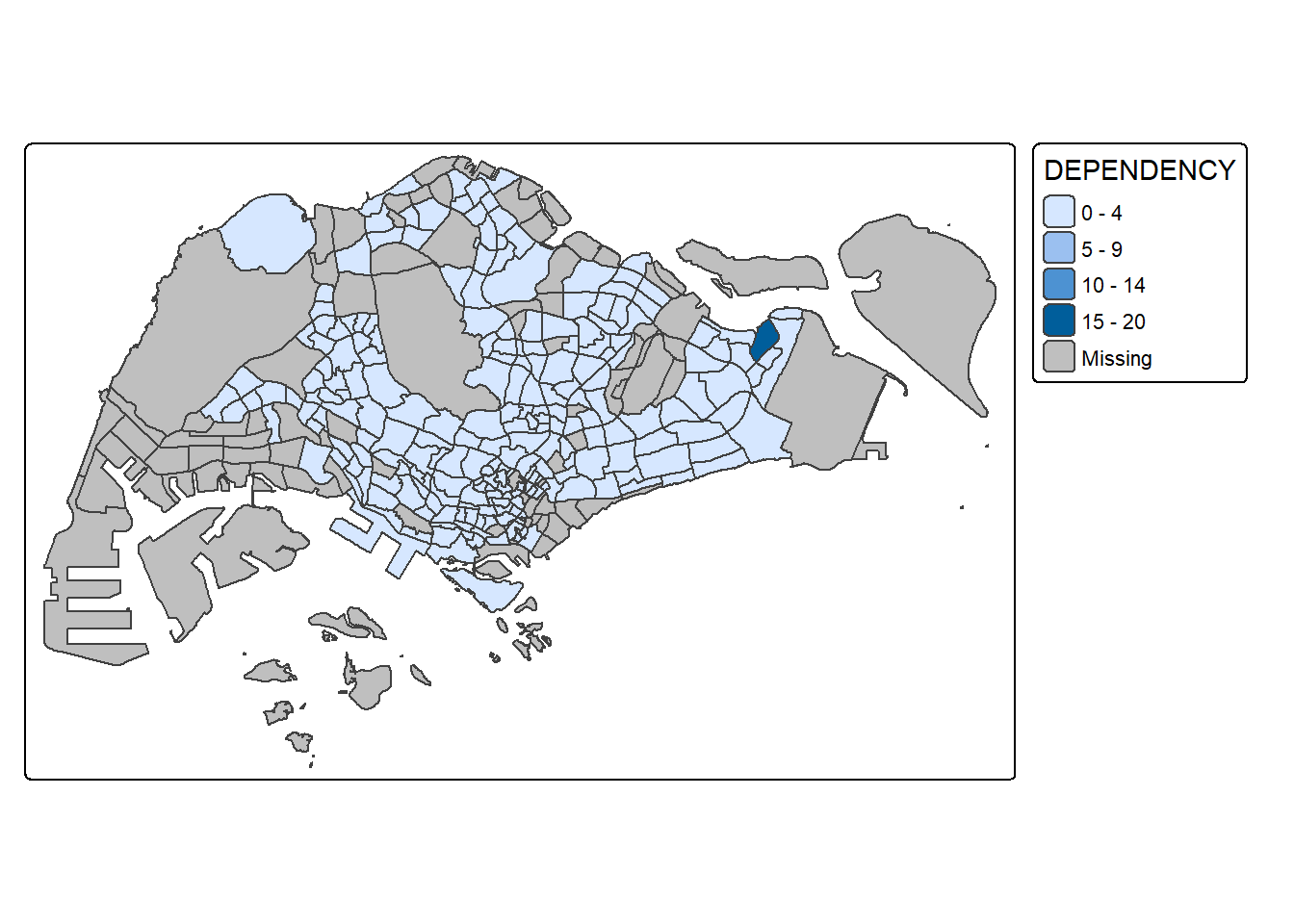
21.4.2.3 Drawing a choropleth map using tm_fill() and *tm_border()**
Without line border
tm_shape(mpsz_pop2020)+
  tm_fill("DEPENDENCY")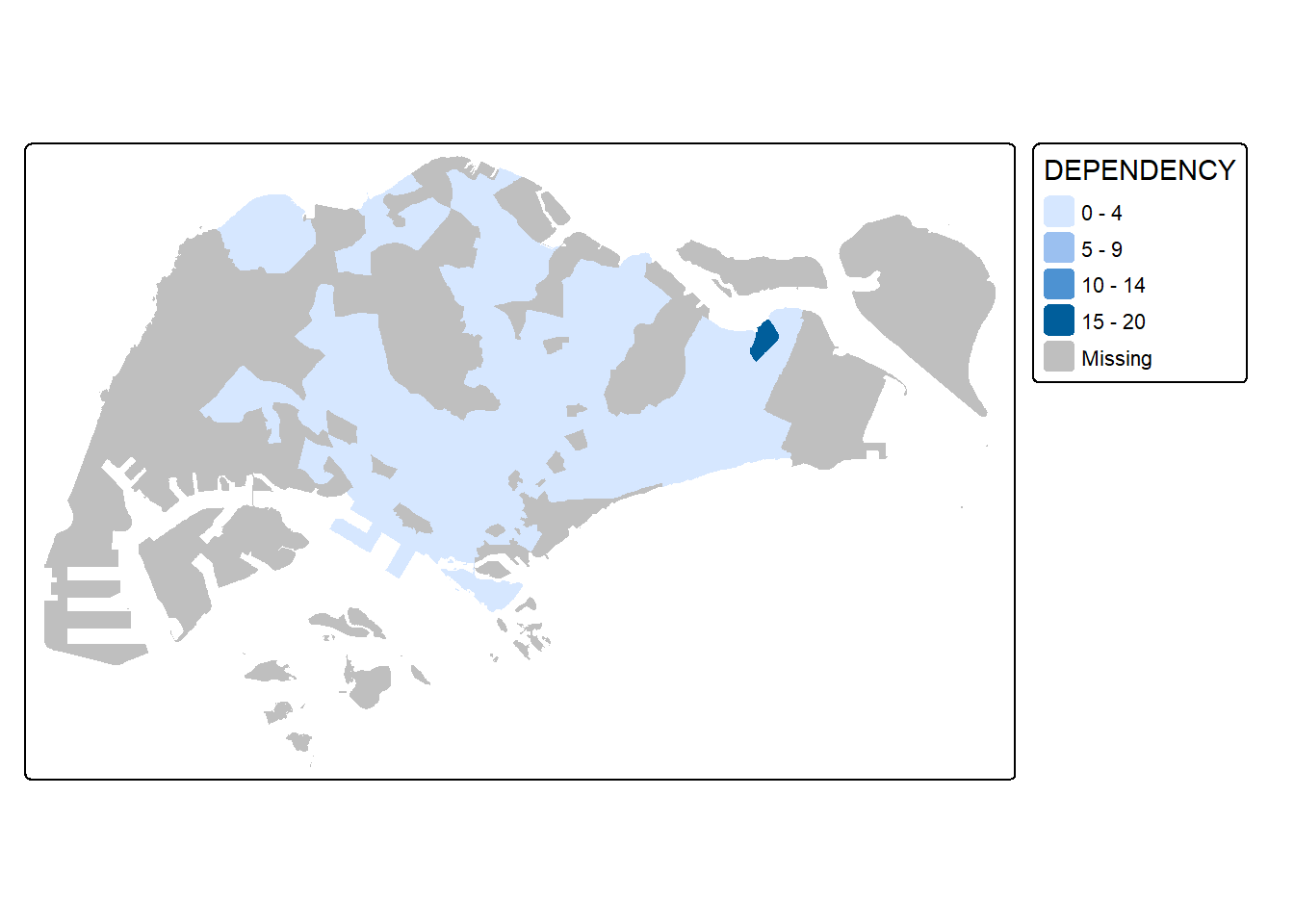
tm_shape(mpsz_pop2020)+
  tm_polygons(fill = "DEPENDENCY") +
  tm_borders(lwd = 0.01,
             fill_alpha = 0.1)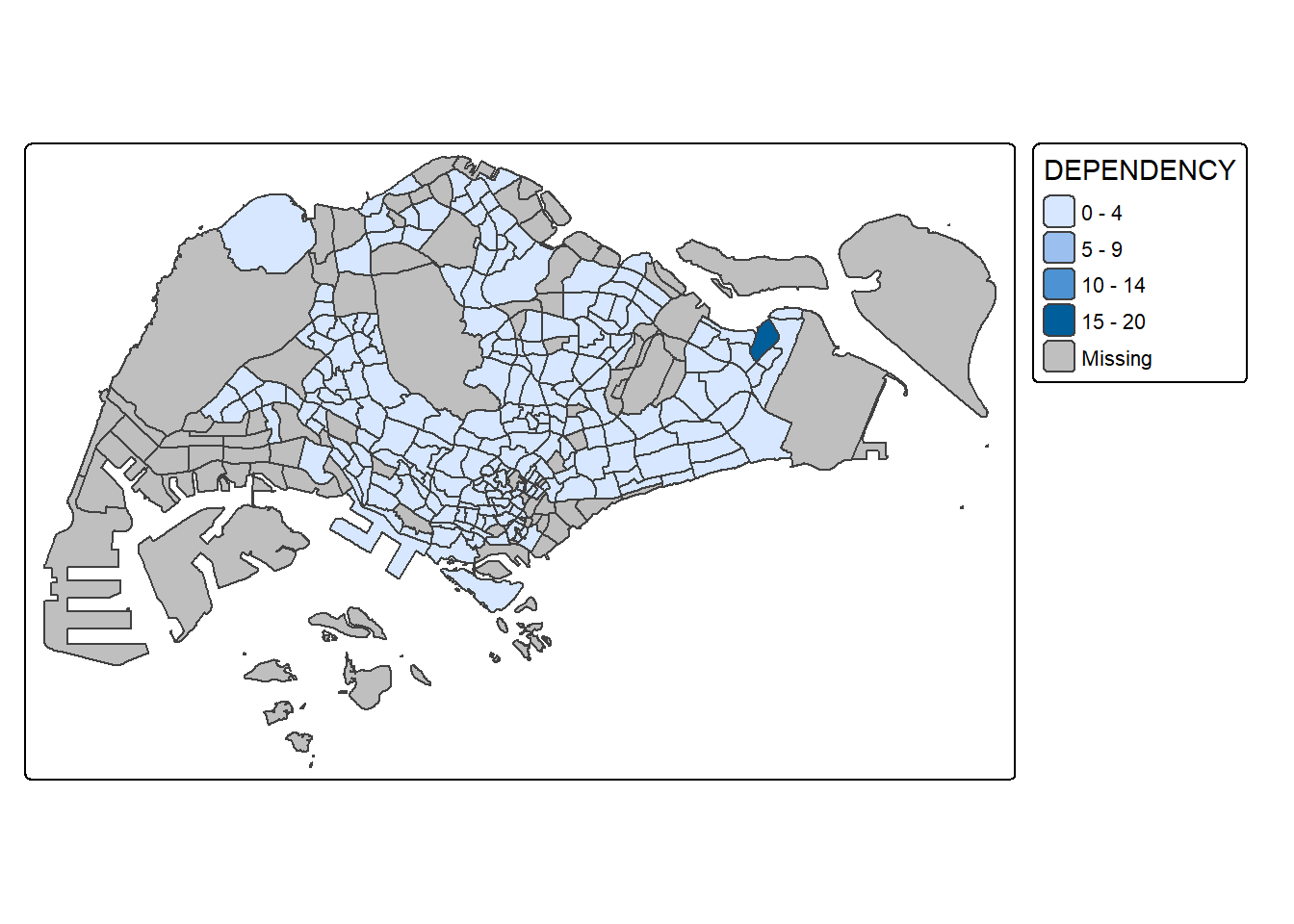
The alpha argument is used to define transparency number between 0 (totally transparent) and 1 (not transparent). By default, the alpha value of the col is used (normally 1).
Beside alpha argument, there are three other arguments for tm_borders(), they are:
col = border colour,
lwd = border line width. The default is 1, and
lty = border line type. The default is “solid”.
21.4.3 Data classification methods of tmap
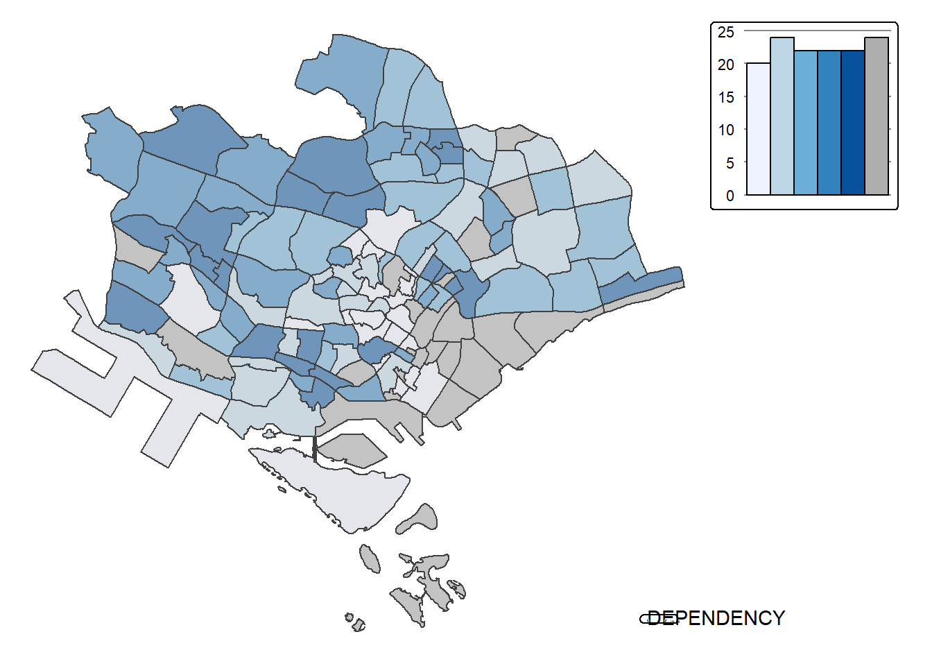
tmap provides a total ten data classification methods, namely: fixed, sd, equal, pretty (default), quantile, kmeans, hclust, bclust, fisher, and jenks.
To define a data classification method, the style argument of tm_fill() or tm_polygons() will be used.
21.4.3.1 Plotting choropleth maps with built-in classification methods
Style=jenks
tm_shape(mpsz_pop2020)+
  tm_polygons("DEPENDENCY",
      fill.scale = tm_scale_intervals(
        style = "jenks",
        n = 5)) +
  tm_borders(fill_alpha = 0.5)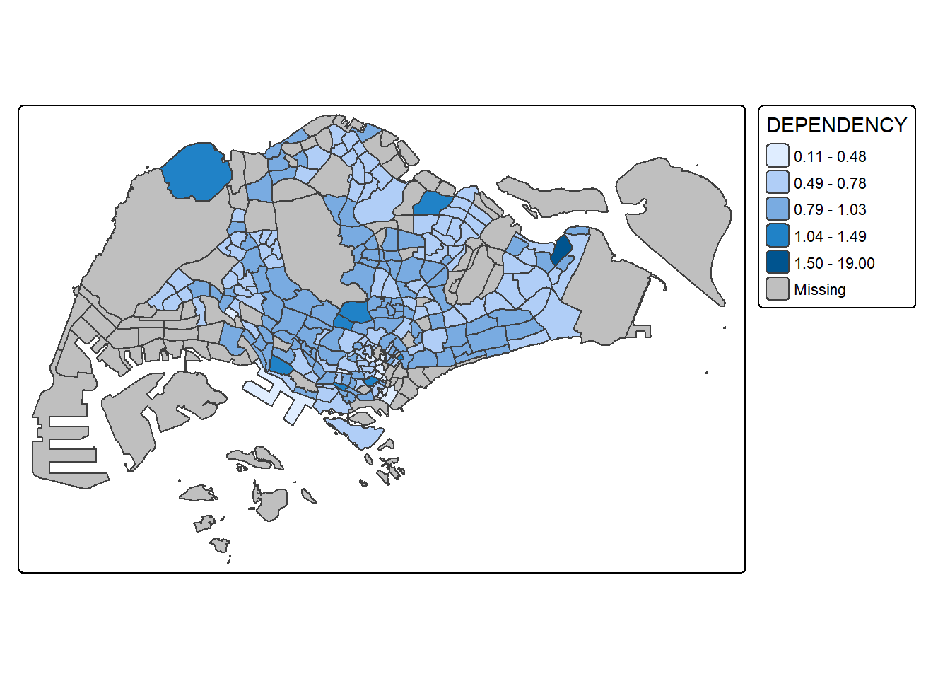
Style=equal
tm_shape(mpsz_pop2020)+
  tm_polygons("DEPENDENCY",
      fill.scale = tm_scale_intervals(
        style = "equal",
        n = 5)) +
  tm_borders(fill_alpha = 0.5)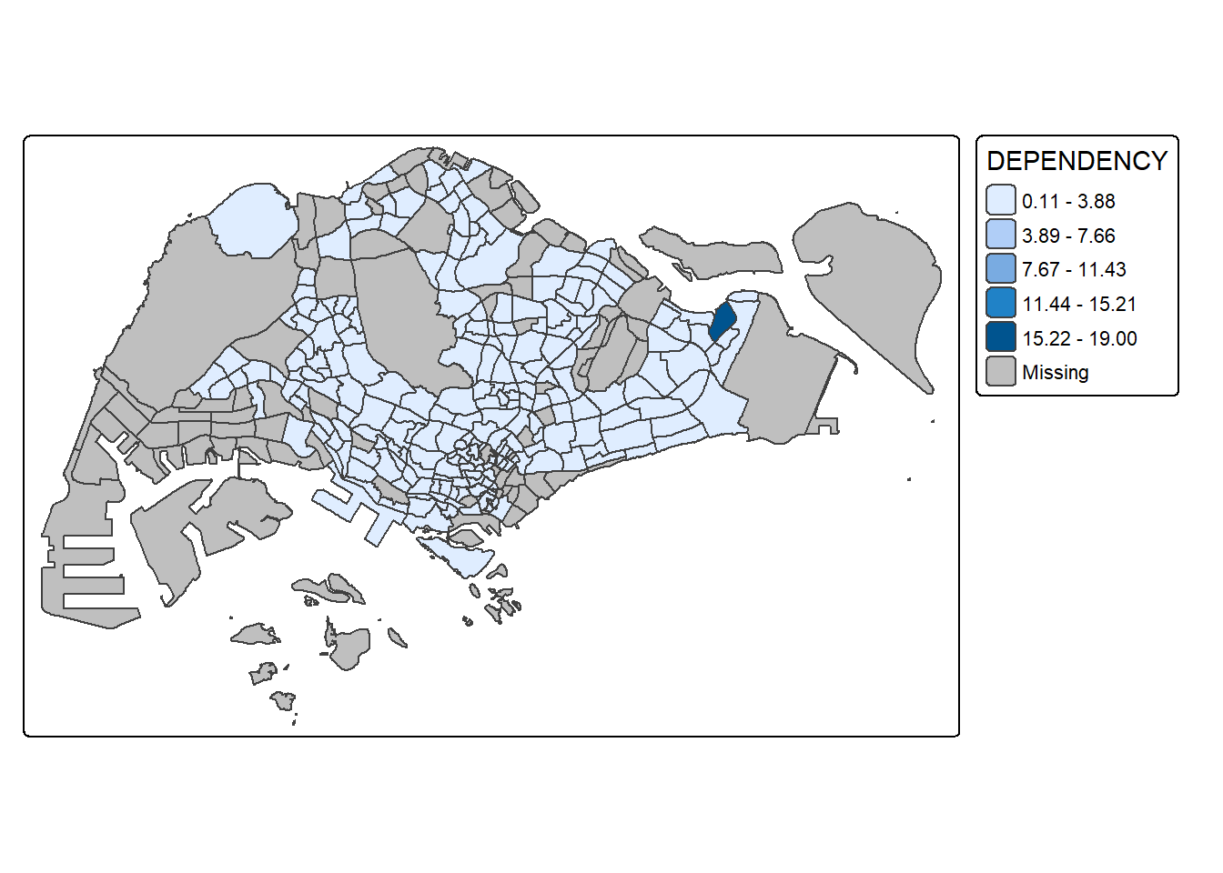
21.4.3.2 Plotting choropleth map with customer break
summary(mpsz_pop2020$DEPENDENCY) Min. 1st Qu. Median Mean 3rd Qu. Max. NA's
0.1111 0.7147 0.7867 0.8585 0.8763 19.0000 92 tm_shape(mpsz_pop2020)+
tm_polygons("DEPENDENCY",
breaks = c(0, 0.60, 0.70, 0.80, 0.90, 1.00)) +
tm_borders(fill_alpha = 0.5)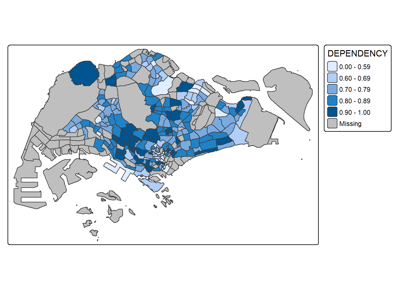
21.4.4 Colour Scheme
21.4.4.1 Using ColourBrewer palette
tm_shape(mpsz_pop2020)+
  tm_polygons("DEPENDENCY",
      fill.scale = tm_scale_intervals(
        style = "quantile",
        n = 5,
        values = "brewer.greens")) +
  tm_borders(fill_alpha = 0.5)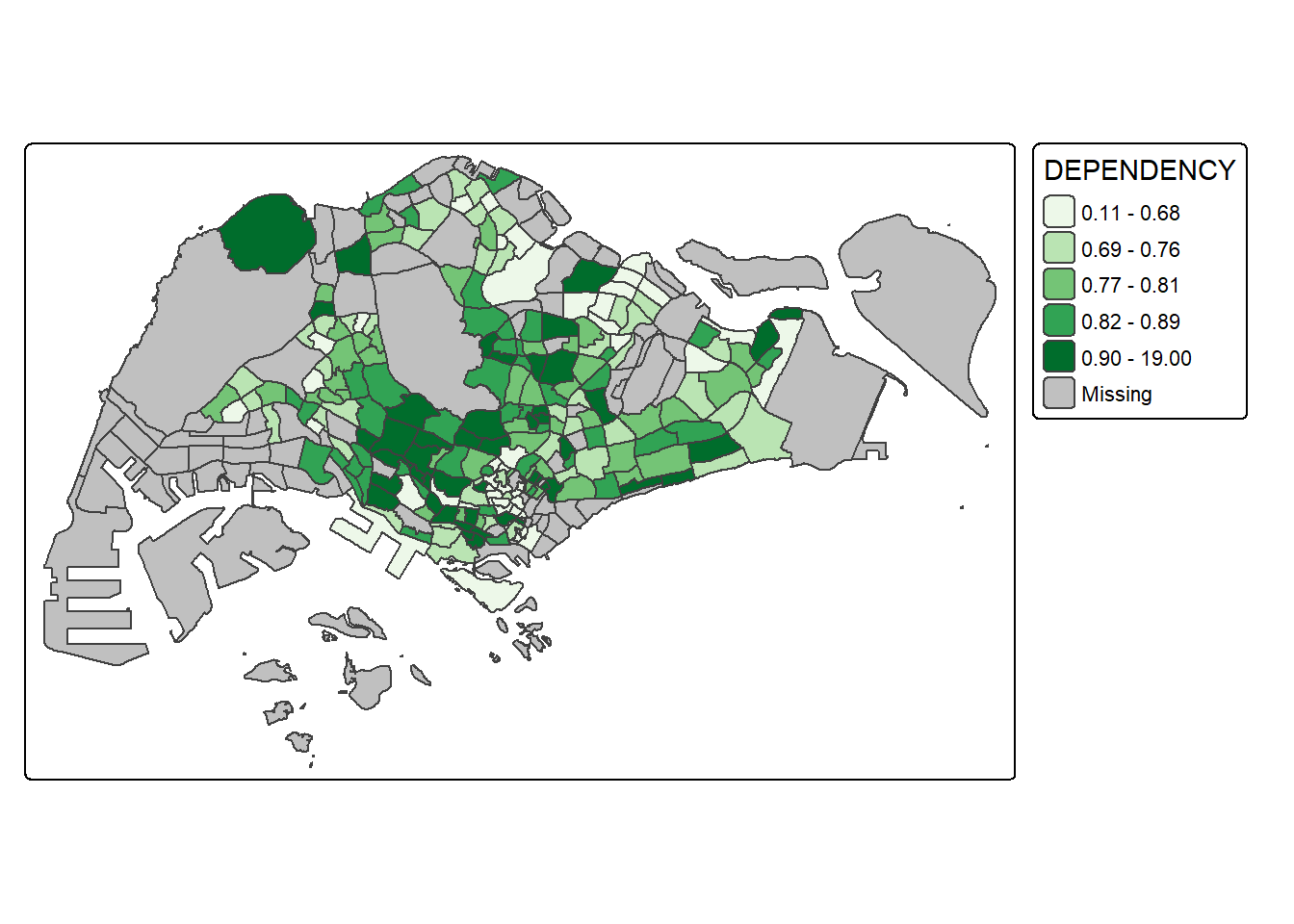
tm_shape(mpsz_pop2020)+
  tm_polygons("DEPENDENCY",
      fill.scale = tm_scale_intervals(
        style = "quantile",
        n = 5,
        values = "-brewer.greens")) +
  tm_borders(fill_alpha = 0.5)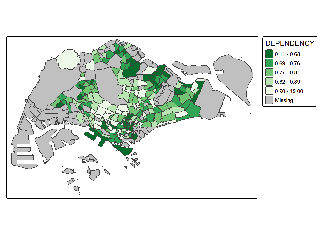
21.4.5 Map Layouts
21.4.5.1 Map Legend
tm_shape(mpsz_pop2020)+
  tm_polygons("DEPENDENCY",
      fill.scale = tm_scale_intervals(
        style = "jenks",
        n = 5,
        values = "brewer.greens"),
      fill.legend = tm_legend(
        title = "Dependency ratio")) +
  tm_borders(fill_alpha = 0.5) +
  tm_title("Distribution of Dependency Ratio by planning subzone \n(Jenks classification)")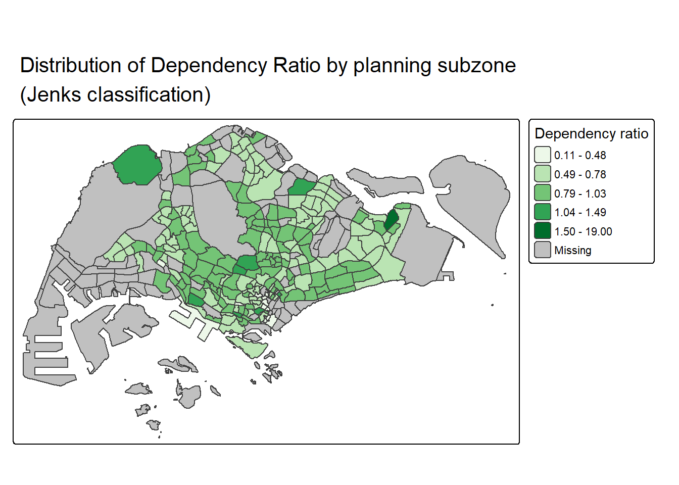
21.4.5.2 Map style
tmap allows a wide variety of layout settings to be changed. They can be called by using tmap_style().
tm_shape(mpsz_pop2020)+
  tm_fill("DEPENDENCY",
          style = "quantile",
          palette = "-Greens") +
  tm_borders(alpha = 0.5) +
  tmap_style("classic")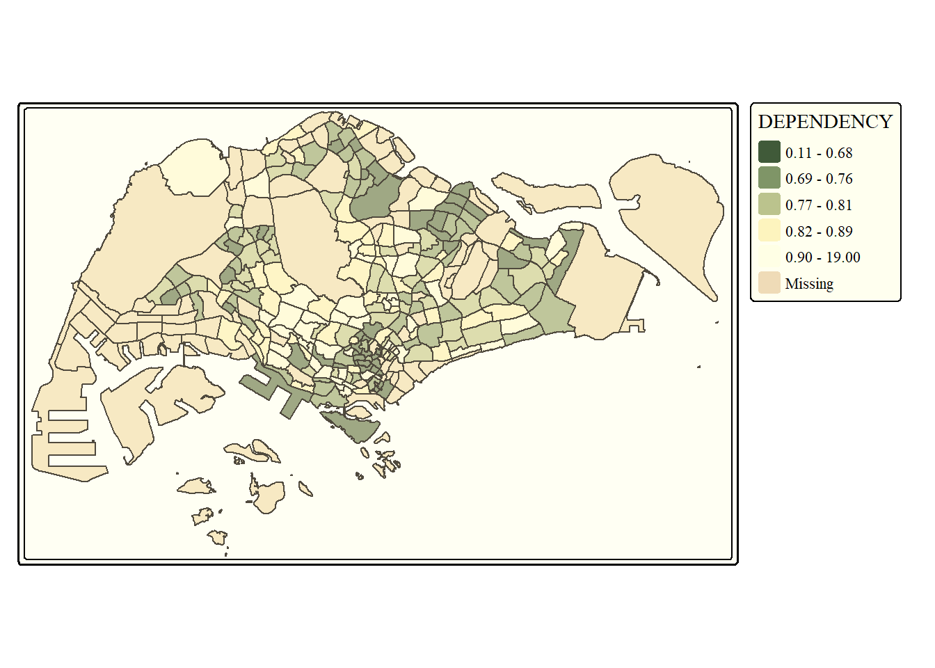
21.4.5.3 Cartographic Furniture
Beside map style, tmap also also provides arguments to draw other map furniture such as compass, scale bar and grid lines.
In the code chunk below, tm_compass(), tm_scale_bar() and tm_grid() are used to add compass, scale bar and grid lines onto the choropleth map.
tm_shape(mpsz_pop2020)+
  tm_polygons(fill = "DEPENDENCY",
              fill.scale = tm_scale_intervals(
                style = "quantile",
                n = 5,
                values = "brewer.blues"),
              fill.legend = tm_legend(
                title = "Dependency ratio")) +
  tm_title("Distribution of Dependency Ratio by planning subzone") +
  tm_layout(frame = TRUE) +
  tm_borders(fill_alpha = 0.5) +
  tm_compass(type="8star", size = 2) +
  tm_grid(alpha =0.2) +
  tm_credits("Source: Planning Sub-zone boundary from Urban Redevelopment Authorithy (URA)\n and Population data from Department of Statistics DOS",
             position = c("left", "bottom"))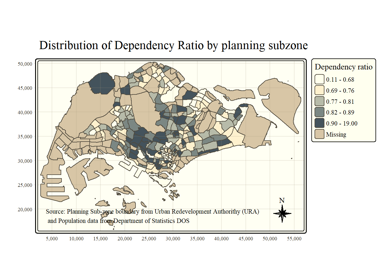
To reset to default stype
tmap_style("white")21.4.6 Drawing Small Multiple Choropleth Maps
21.4.6.1 By assigning multiple values to at least one of the aesthetic arguments
tm_shape(mpsz_pop2020)+
  tm_fill(c("YOUNG", "AGED"),
          style = "equal",
          palette = "Blues",
          ncols = 1) +
  tm_layout(legend.position = c("right", "bottom")) +
  tm_borders(alpha = 0.5) +
  tmap_style("white")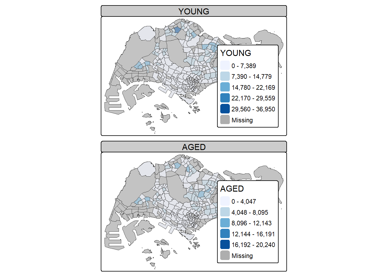
tm_shape(mpsz_pop2020)+
  tm_polygons(c("DEPENDENCY","AGED"),
          style = c("equal", "quantile"),
          palette = list("Blues","Greens")) +
  tm_layout(legend.position = c("right", "bottom"))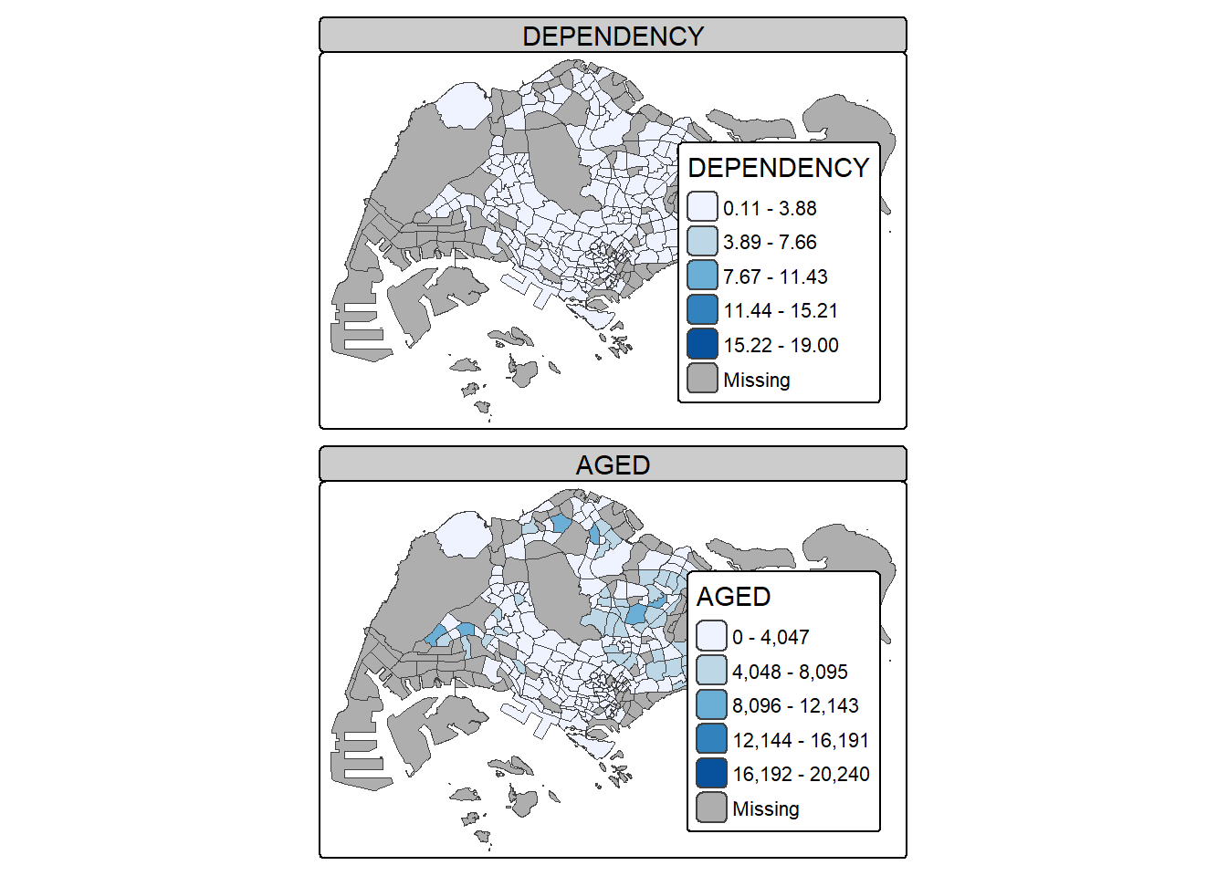
tm_shape(mpsz_pop2020)+
  tm_polygons(c("DEPENDENCY","AGED"),
          style = c("equal", "quantile"),
          palette = list("Blues","Greens")) +
  tm_layout(legend.position = c("right", "bottom"))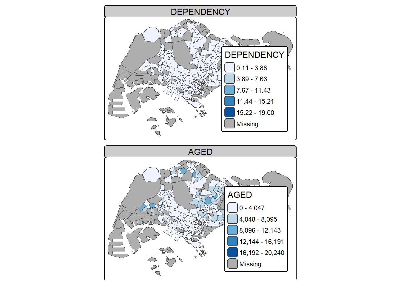
21.4.6.2 By defining a group-by variable in tm_facets()
Multiple small choropleth maps are created by using tm_facets().
tm_shape(mpsz_pop2020) +
  tm_fill("DEPENDENCY",
          style = "quantile",
          palette = "Blues",
          thres.poly = 0) +
  tm_facets(by="REGION_N",
            free.coords=TRUE) +
  tm_layout(legend.show = FALSE,
            title.position = c("center", "center"),
            title.size = 20) +
  tm_borders(alpha = 0.5)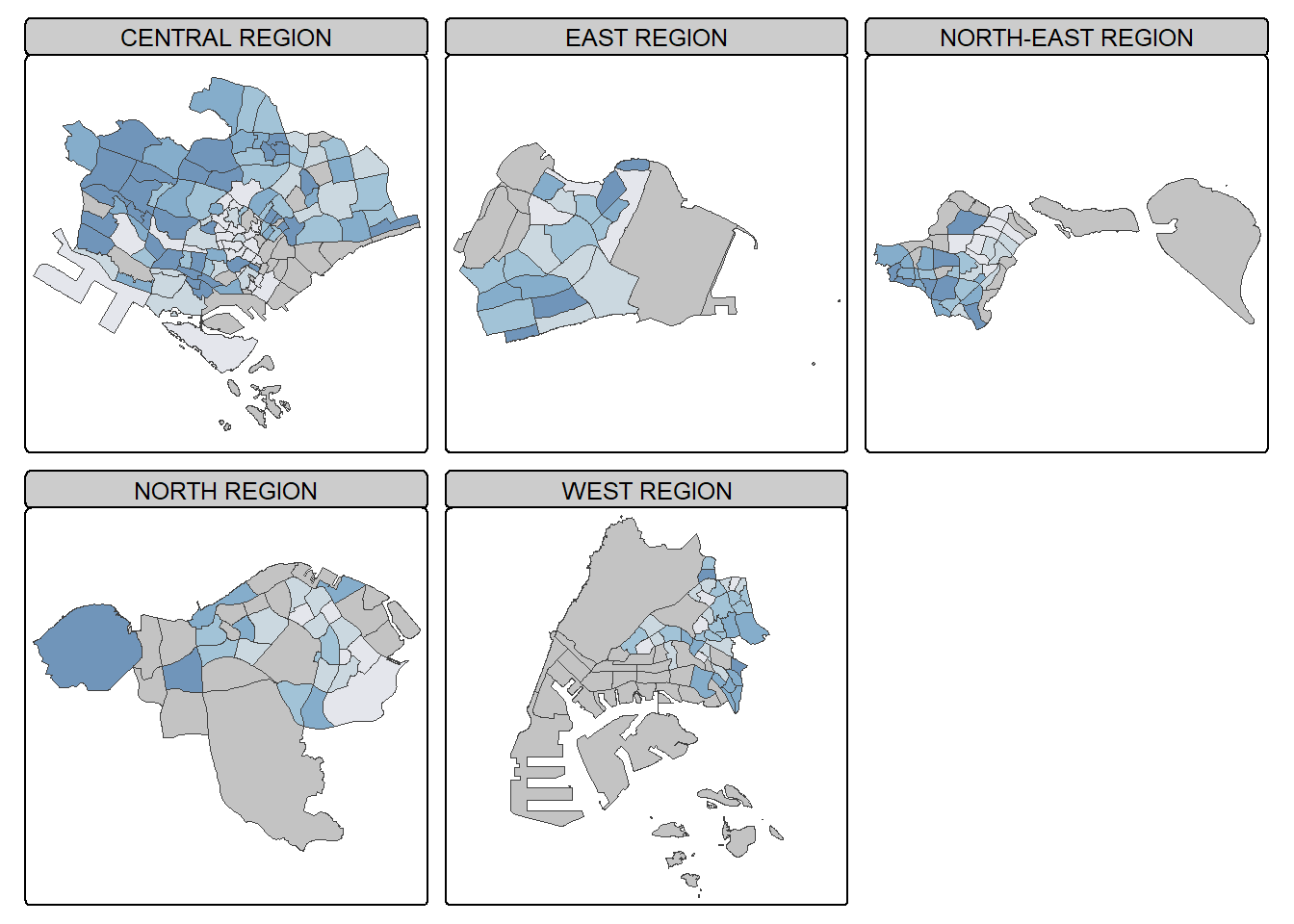
21.4.6.3 By creating multiple stand-alone maps with tmap_arrange()
youngmap <- tm_shape(mpsz_pop2020)+
  tm_polygons("YOUNG",
              style = "quantile",
              palette = "Blues")

agedmap <- tm_shape(mpsz_pop2020)+
  tm_polygons("AGED",
              style = "quantile",
              palette = "Blues")

tmap_arrange(youngmap, agedmap, asp=1, ncol=2)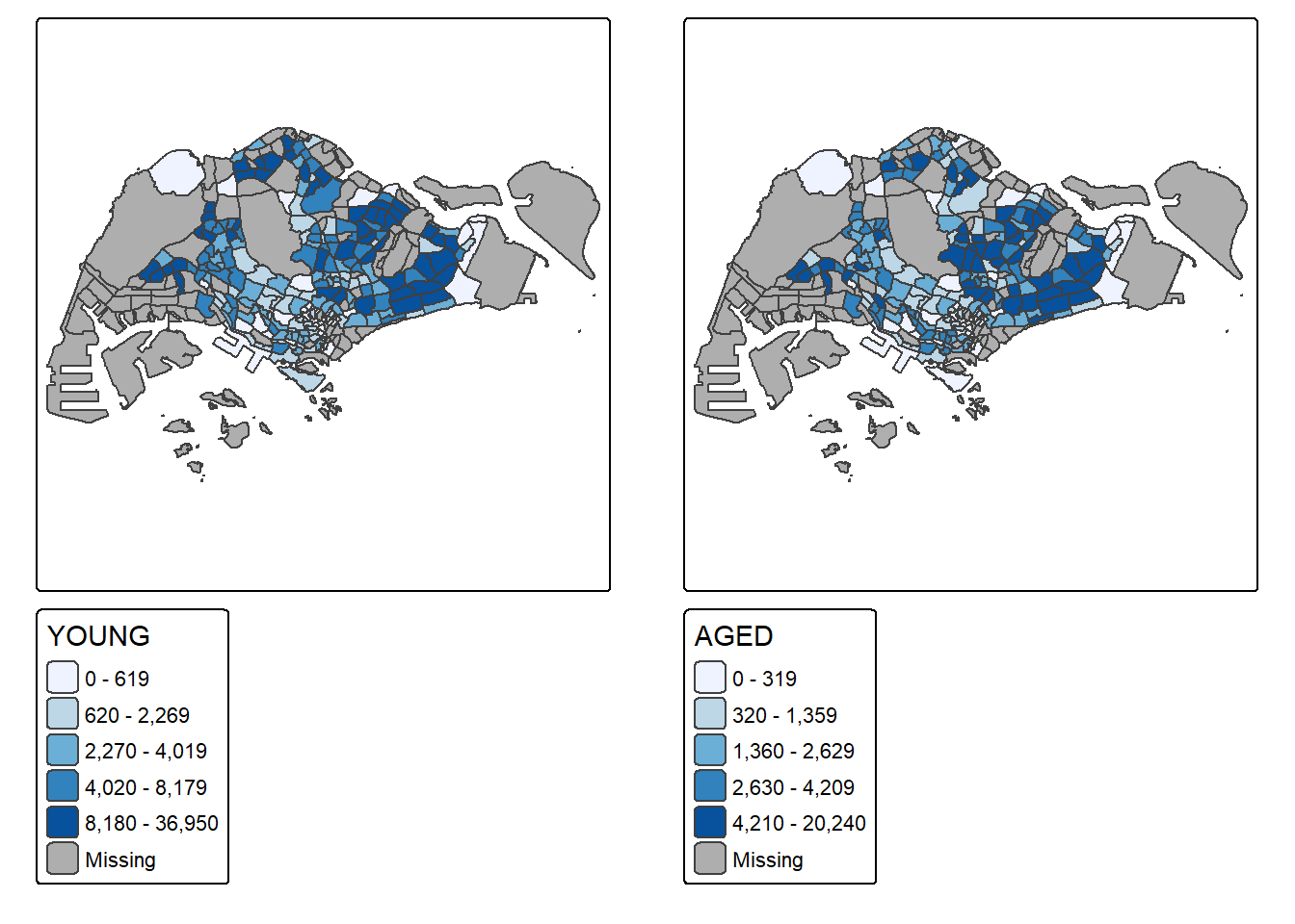
21.4.7 Mappping Spatial Object Meeting a Selection Criterion
tm_shape(mpsz_pop2020[mpsz_pop2020$REGION_N=="CENTRAL REGION", ])+
  tm_fill("DEPENDENCY",
          style = "quantile",
          palette = "Blues",
          legend.hist = TRUE,
          legend.is.portrait = TRUE,
          legend.hist.z = 0.1) +
  tm_layout(legend.outside = TRUE,
            legend.height = 0.45,
            legend.width = 2,
            legend.position = c("right", "bottom"),
            legend.outside = TRUE,
            legend.outside.position = "right",
            frame = FALSE) +
  tm_borders(alpha = 0.5)