pacman::p_load(treemap, treemapify, tidyverse) Hands-on_EX05e
16 Treemap Visualisation with R
16.2 Installing and Launching R Packages
16.3 Data Wrangling
16.3.1 Importing the data set
realis2018 <- read_csv("data/realis2018.csv")16.3.2 Data Wrangling and Manipulation
In this section, we will perform the following steps to manipulate and prepare a data.frtame that is appropriate for treemap visualisation:
group transaction records by Project Name, Planning Region, Planning Area, Property Type and Type of Sale, and
compute Total Unit Sold, Total Area, Median Unit Price and Median Transacted Price by applying appropriate summary statistics on No. of Units, Area (sqm), Unit Price ($ psm) and Transacted Price ($) respectively.
Grouping [group_by() and summarize()] affects the verbs as follows:
grouped select() is the same as ungrouped select(), except that grouping variables are always retained.
grouped arrange() is the same as ungrouped; unless you set .by_group = TRUE, in which case it orders first by the grouping variables.
mutate() and filter() are most useful in conjunction with window functions (like rank(), or min(x) == x). They are described in detail in vignette(“window-functions”).
sample_n() and sample_frac() sample the specified number/fraction of rows in each group.
summarise() computes the summary for each group.
16.3.3 Grouped summaries without the Pipe
realis2018_grouped <- group_by(realis2018, `Project Name`,
                               `Planning Region`, `Planning Area`,
                               `Property Type`, `Type of Sale`)
realis2018_summarised <- summarise(realis2018_grouped,
                          `Total Unit Sold` = sum(`No. of Units`, na.rm = TRUE),
                          `Total Area` = sum(`Area (sqm)`, na.rm = TRUE),
                          `Median Unit Price ($ psm)` = median(`Unit Price ($ psm)`, na.rm = TRUE),
                          `Median Transacted Price` = median(`Transacted Price ($)`, na.rm = TRUE))
`summarise()` has regrouped the output.
ℹ Summaries were computed grouped by Project Name, Planning Region, Planning
Area, Property Type, and Type of Sale.
ℹ Output is grouped by Project Name, Planning Region, Planning Area, and
Property Type.
ℹ Use `summarise(.groups = "drop_last")` to silence this message.
ℹ Use `summarise(.by = c(Project Name, Planning Region, Planning Area, Property
Type, Type of Sale))` for per-operation grouping (`?dplyr::dplyr_by`)
instead.Aggregation functions such as sum() and meadian() obey the usual rule of missing values: if there’s any missing value in the input, the output will be a missing value. The argument na.rm = TRUE removes the missing values prior to computation
16.4 Designing Treemap with treemap Package
16.4.1 Designing a static treemap
realis2018_selected <- realis2018_summarised %>%
  filter(`Property Type` == "Condominium", `Type of Sale` == "Resale")
16.4.2 Using the basic arguments
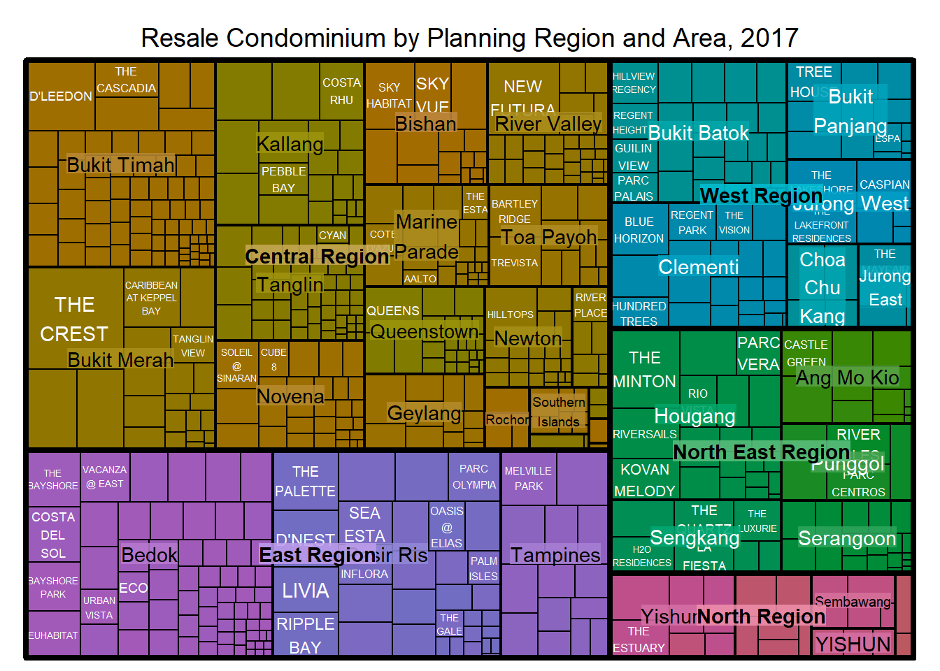
index
The index vector must consist of at least two column names or else no hierarchy treemap will be plotted.
If multiple column names are provided, such as the code chunk above, the first name is the highest aggregation level, the second name the second highest aggregation level, and so on.
vSize
- The column must not contain negative values. This is because it’s vaues will be used to map the sizes of the rectangles of the treemaps.
treemap(realis2018_selected,
        index=c("Planning Region", "Planning Area", "Project Name"),
        vSize="Total Unit Sold",
        vColor="Median Unit Price ($ psm)",
        title="Resale Condominium by Planning Region and Area, 2017",
        title.legend = "Median Unit Price (S$ per sq. m)"
        )
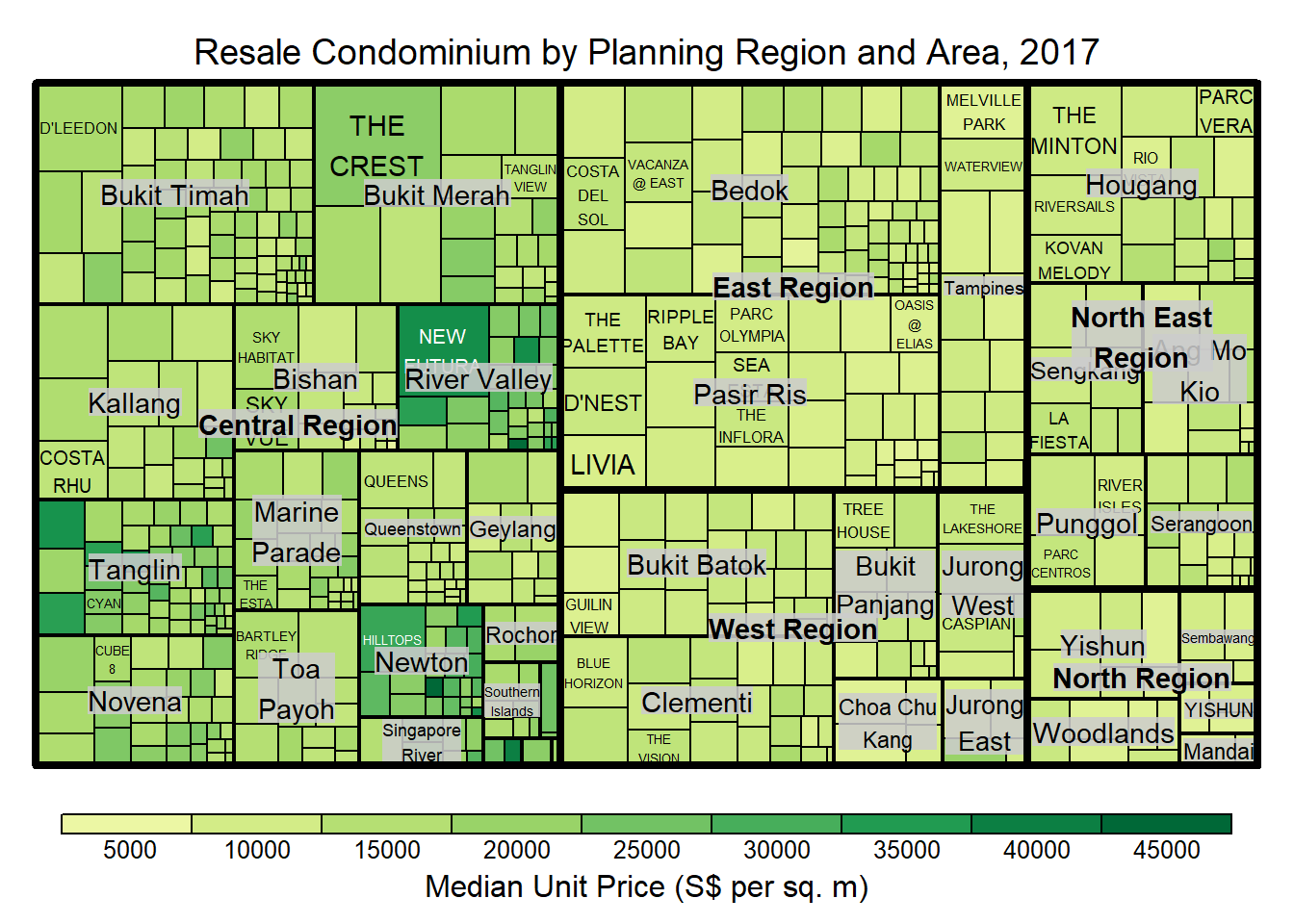
16.4.3 Working with vColor and type arguments
treemap(realis2018_selected,
        index=c("Planning Region", "Planning Area", "Project Name"),
        vSize="Total Unit Sold",
        vColor="Median Unit Price ($ psm)",
        type = "value",
        title="Resale Condominium by Planning Region and Area, 2017",
        title.legend = "Median Unit Price (S$ per sq. m)"
        )
16.4.4 Colours in treemap package
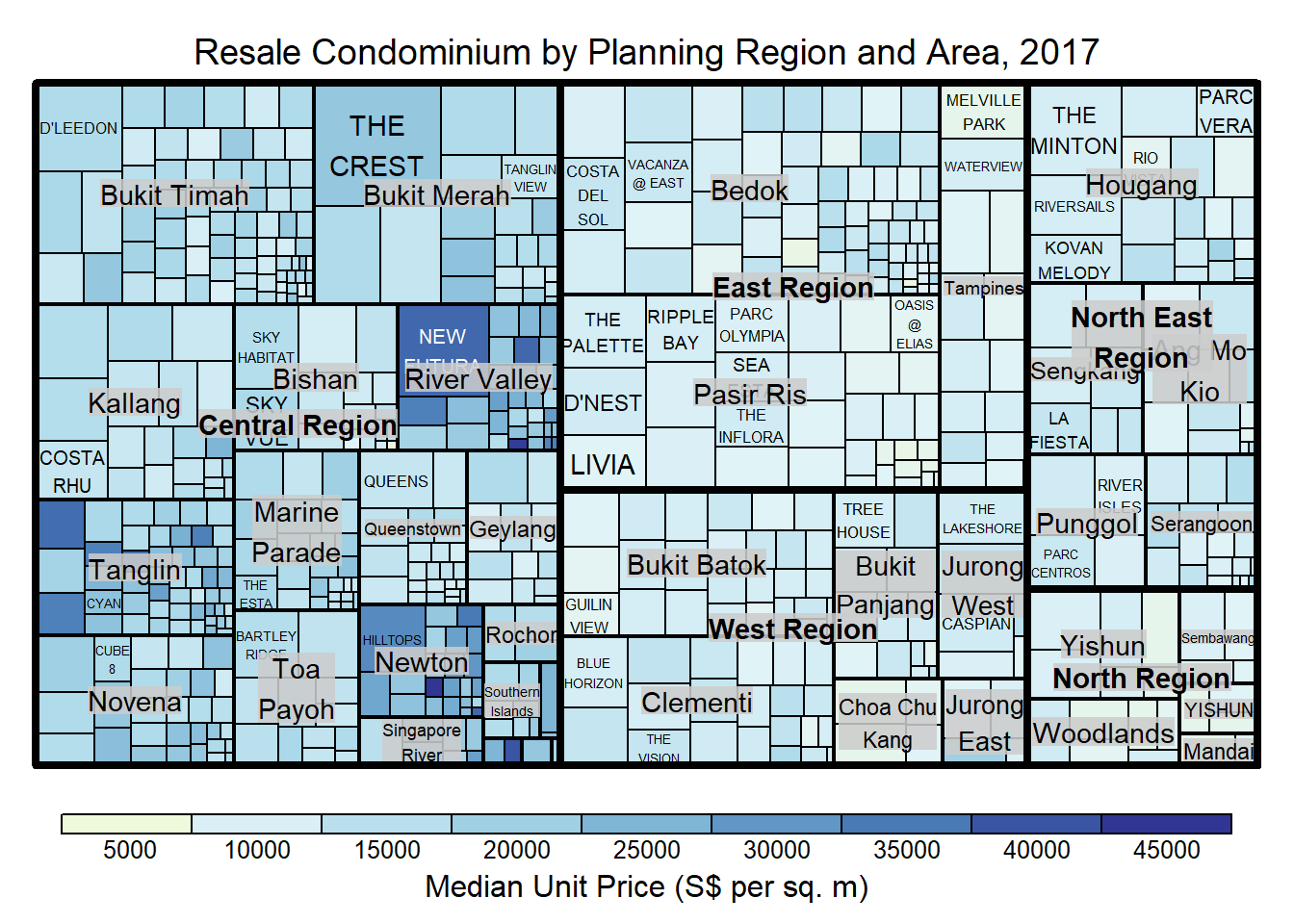
The “value” treemap considers palette to be a diverging color palette (say ColorBrewer’s “RdYlBu”), and maps it in such a way that 0 corresponds to the middle color (typically white or yellow), -max(abs(values)) to the left-end color, and max(abs(values)), to the right-end color.
The “manual” treemap simply maps min(values) to the left-end color, max(values) to the right-end color, and mean(range(values)) to the middle color.
16.4.5 The “value” type treemap
treemap(realis2018_selected,
        index=c("Planning Region", "Planning Area", "Project Name"),
        vSize="Total Unit Sold",
        vColor="Median Unit Price ($ psm)",
        type="value",
        palette="RdYlBu",
        title="Resale Condominium by Planning Region and Area, 2017",
        title.legend = "Median Unit Price (S$ per sq. m)"
        )
16.4.6 The “manual” type treemap
treemap(realis2018_selected,
        index=c("Planning Region", "Planning Area", "Project Name"),
        vSize="Total Unit Sold",
        vColor="Median Unit Price ($ psm)",
        type="manual",
        palette="RdYlBu",
        title="Resale Condominium by Planning Region and Area, 2017",
        title.legend = "Median Unit Price (S$ per sq. m)"
        )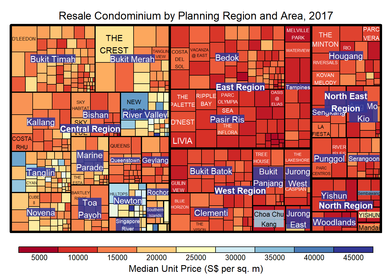
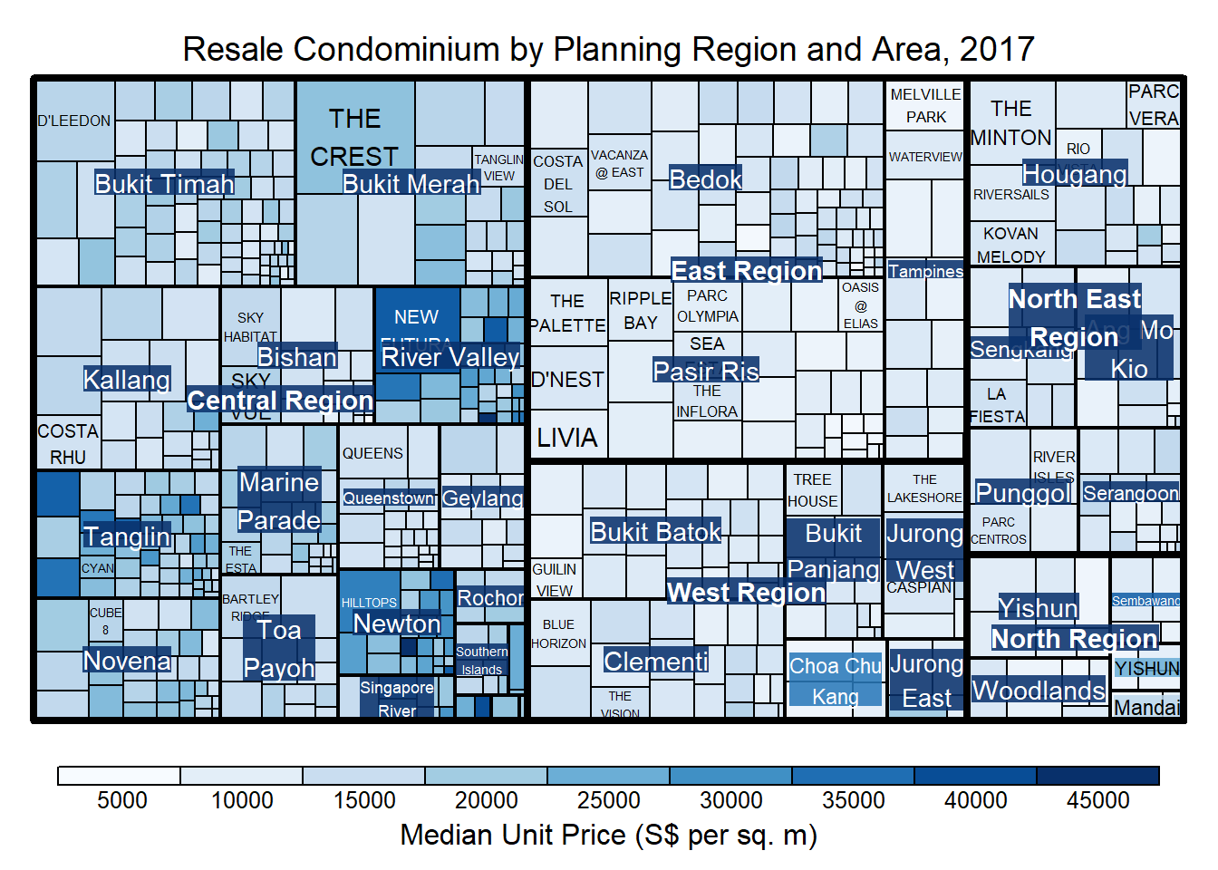
It is not wise to use diverging colour palette such as RdYlBu if the values are all positive or negative
Thus a single colour palette such as Blues should be used
treemap(realis2018_selected,
        index=c("Planning Region", "Planning Area", "Project Name"),
        vSize="Total Unit Sold",
        vColor="Median Unit Price ($ psm)",
        type="manual",
        palette="Blues",
        title="Resale Condominium by Planning Region and Area, 2017",
        title.legend = "Median Unit Price (S$ per sq. m)"
        )
16.4.7 Treemap Layout
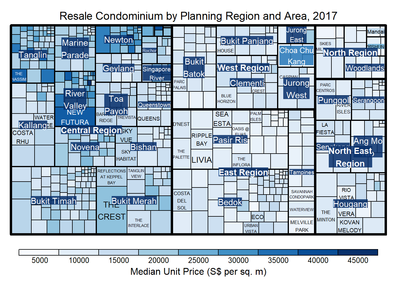
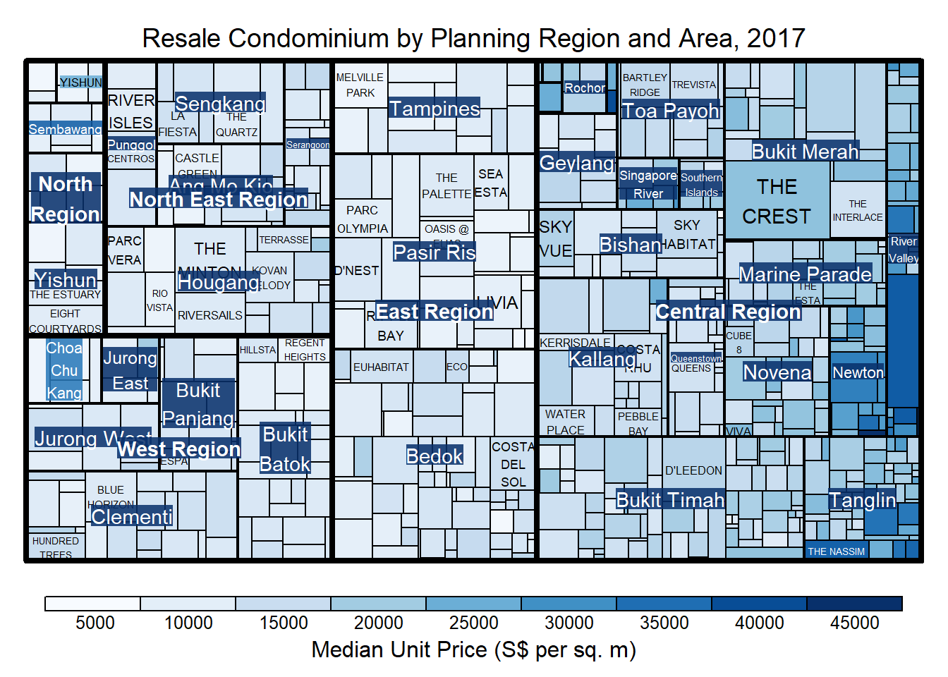
treemap() supports two popular treemap layouts, namely: “squarified” and “pivotSize”. The default is “pivotSize”.
The squarified treemap algorithm (Bruls et al., 2000) produces good aspect ratios, but ignores the sorting order of the rectangles (sortID).
The ordered treemap, pivot-by-size, algorithm (Bederson et al., 2002) takes the sorting order (sortID) into account while aspect ratios are still acceptable.
16.4.8 Working with algorithm argument
Squarified
treemap(realis2018_selected,
        index=c("Planning Region", "Planning Area", "Project Name"),
        vSize="Total Unit Sold",
        vColor="Median Unit Price ($ psm)",
        type="manual",
        palette="Blues",
        algorithm = "squarified",
        title="Resale Condominium by Planning Region and Area, 2017",
        title.legend = "Median Unit Price (S$ per sq. m)"
        )
Pivot Size
treemap(realis2018_selected,
        index=c("Planning Region", "Planning Area", "Project Name"),
        vSize="Total Unit Sold",
        vColor="Median Unit Price ($ psm)",
        type="manual",
        palette="Blues",
        algorithm = "pivotSize",
        sortID = "Median Transacted Price",
        title="Resale Condominium by Planning Region and Area, 2017",
        title.legend = "Median Unit Price (S$ per sq. m)"
        )
16.5 Designing Treemap using treemapify Package
ggplot(data=realis2018_selected,
       aes(area = `Total Unit Sold`,
           fill = `Median Unit Price ($ psm)`),
       layout = "scol",
       start = "bottomleft") +
  geom_treemap() +
  scale_fill_gradient(low = "light blue", high = "blue")
Warning in fortify(data, ...): Arguments in `...` must be used.
✖ Problematic arguments:
• layout = "scol"
• start = "bottomleft"
ℹ Did you misspell an argument name?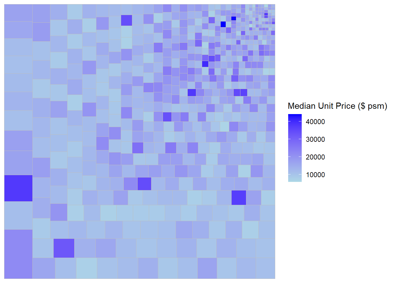
16.5.2 Defining hierarchy
Group by Planning Region
ggplot(data=realis2018_selected,
       aes(area = `Total Unit Sold`,
           fill = `Median Unit Price ($ psm)`,
           subgroup = `Planning Region`),
       start = "topleft") +
  geom_treemap()
Warning in fortify(data, ...): Arguments in `...` must be used.
✖ Problematic argument:
• start = "topleft"
ℹ Did you misspell an argument name?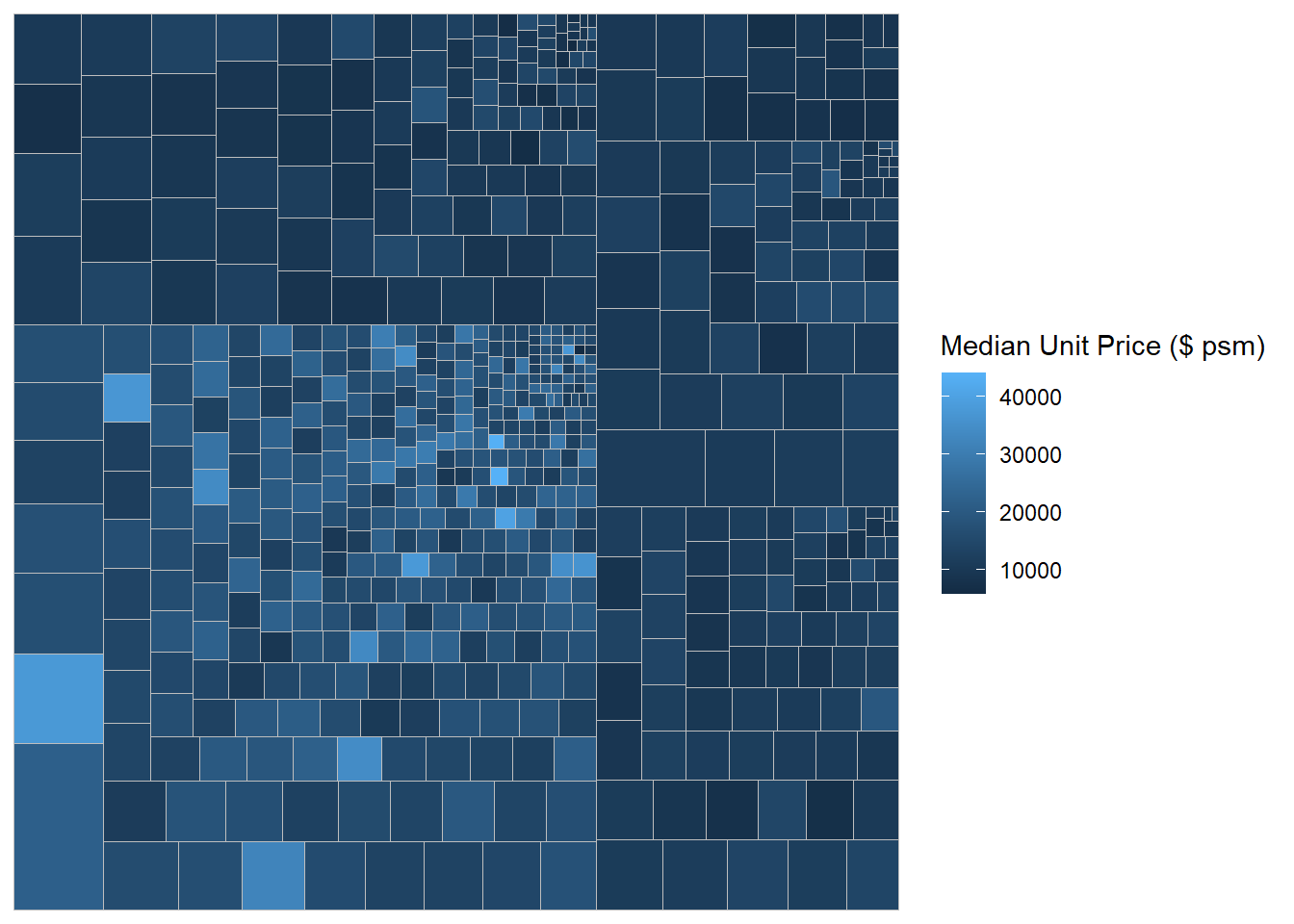
Group by Planning Area
ggplot(data=realis2018_selected,
       aes(area = `Total Unit Sold`,
           fill = `Median Unit Price ($ psm)`,
           subgroup = `Planning Region`,
           subgroup2 = `Planning Area`)) +
  geom_treemap()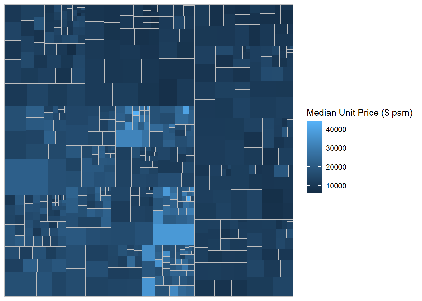
Adding boundary line
ggplot(data=realis2018_selected,
       aes(area = `Total Unit Sold`,
           fill = `Median Unit Price ($ psm)`,
           subgroup = `Planning Region`,
           subgroup2 = `Planning Area`)) +
  geom_treemap() +
  geom_treemap_subgroup2_border(colour = "gray40",
                                size = 2) +
  geom_treemap_subgroup_border(colour = "gray20")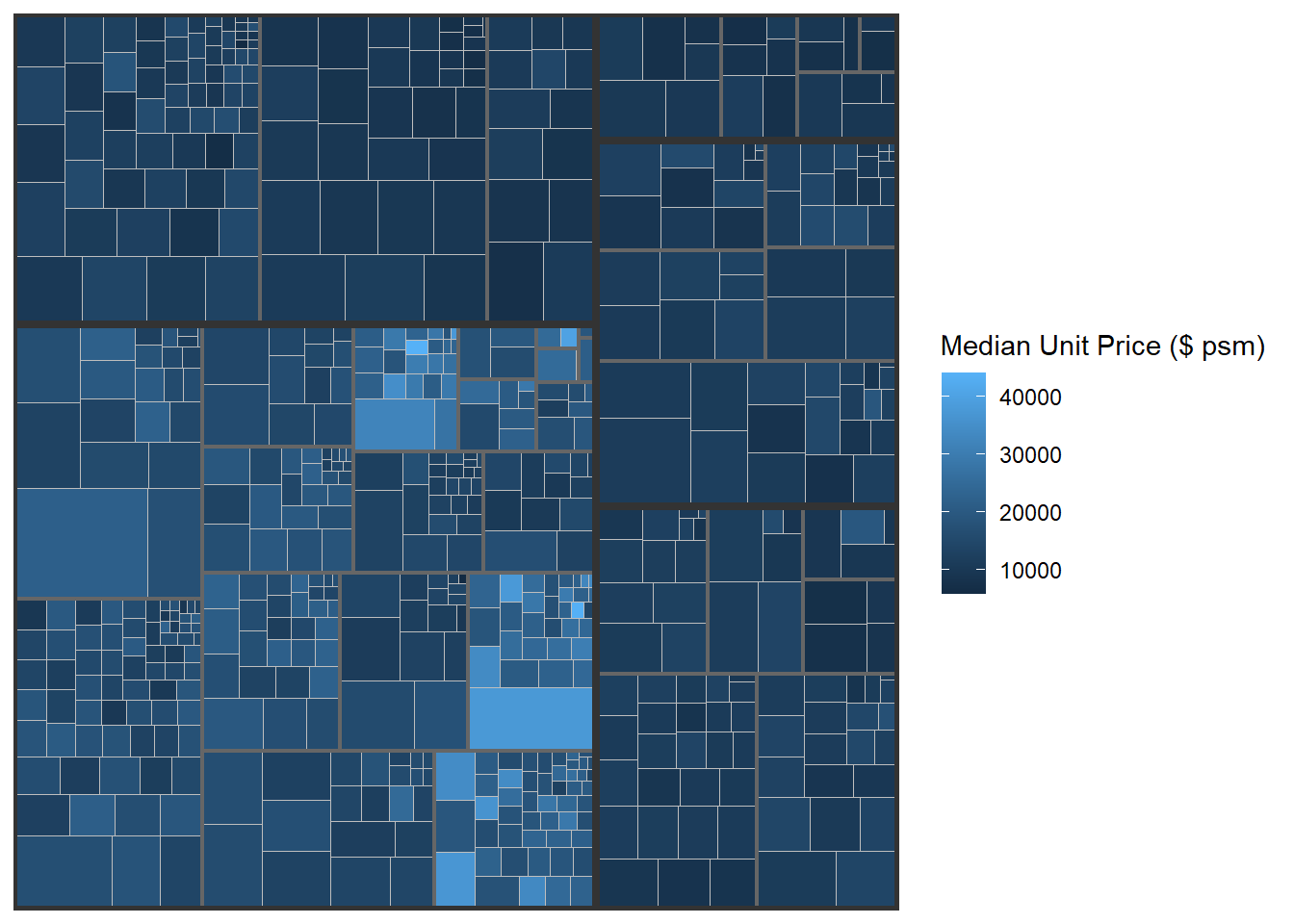
16.6 Designing Interactive Treemap using d3treeR
16.6.1 Installing d3treeR package
- If this is the first time you install a package from github, you should install devtools package by using the code below or else you can skip this step.
install.packages(“devtools”)
- Next, you will load the devtools library and install the package found in github by using the codes below.
library(devtools)Loading required package: usethisinstall_github("timelyportfolio/d3treeR")Using GitHub PAT from the git credential store.Skipping install of 'd3treeR' from a github remote, the SHA1 (ebb833db) has not changed since last install.
Use `force = TRUE` to force installation- Now you are ready to launch d3treeR package
library(d3treeR)16.6.2 Designing An Interactive Treemap
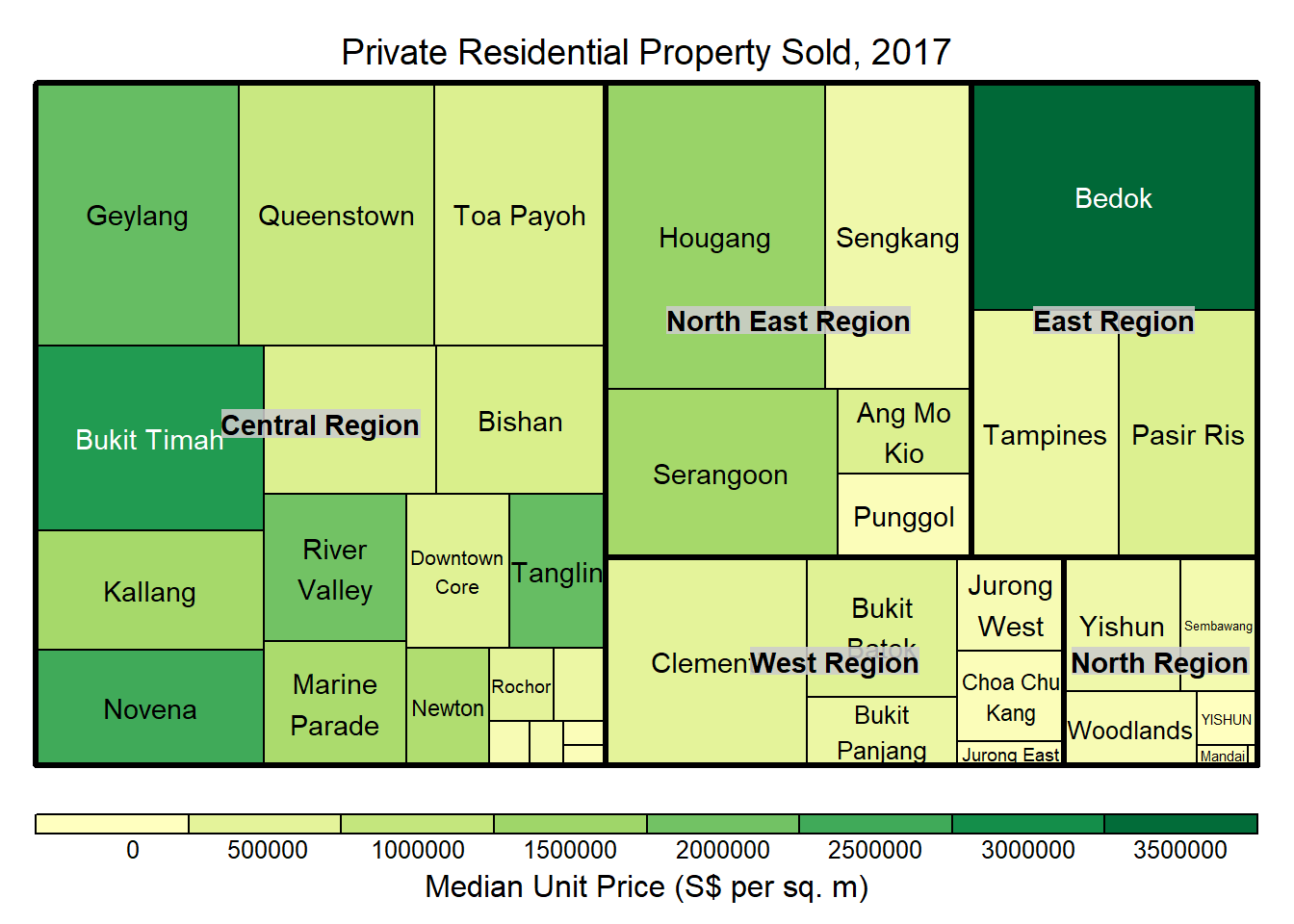
- treemap() is used to build a treemap by using selected variables in condominium data.frame. The treemap created is save as object called tm.
tm <- treemap(realis2018_summarised,
        index=c("Planning Region", "Planning Area"),
        vSize="Total Unit Sold",
        vColor="Median Unit Price ($ psm)",
        type="value",
        title="Private Residential Property Sold, 2017",
        title.legend = "Median Unit Price (S$ per sq. m)"
        )
- Then d3tree() is used to build an interactive treemap.
d3tree(tm,rootname = "Singapore" )