Hands-on_Ex04b

10  Visual Statistical Analysis

10.3 Getting Started

10.3.1 Installing and launching R packages

pacman::p_load(ggstatsplot, tidyverse)

10.3.2 Importing data

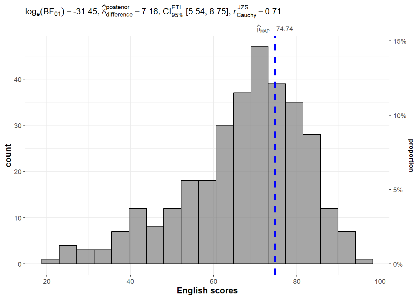
exam <- read_csv("data/Exam_data.csv")

10.3.3 One-sample test: gghistostats() method

set.seed(1234)

gghistostats(
  data = exam,
  x = ENGLISH,
  type = "bayes",
  test.value = 60,
  xlab = "English scores"
)

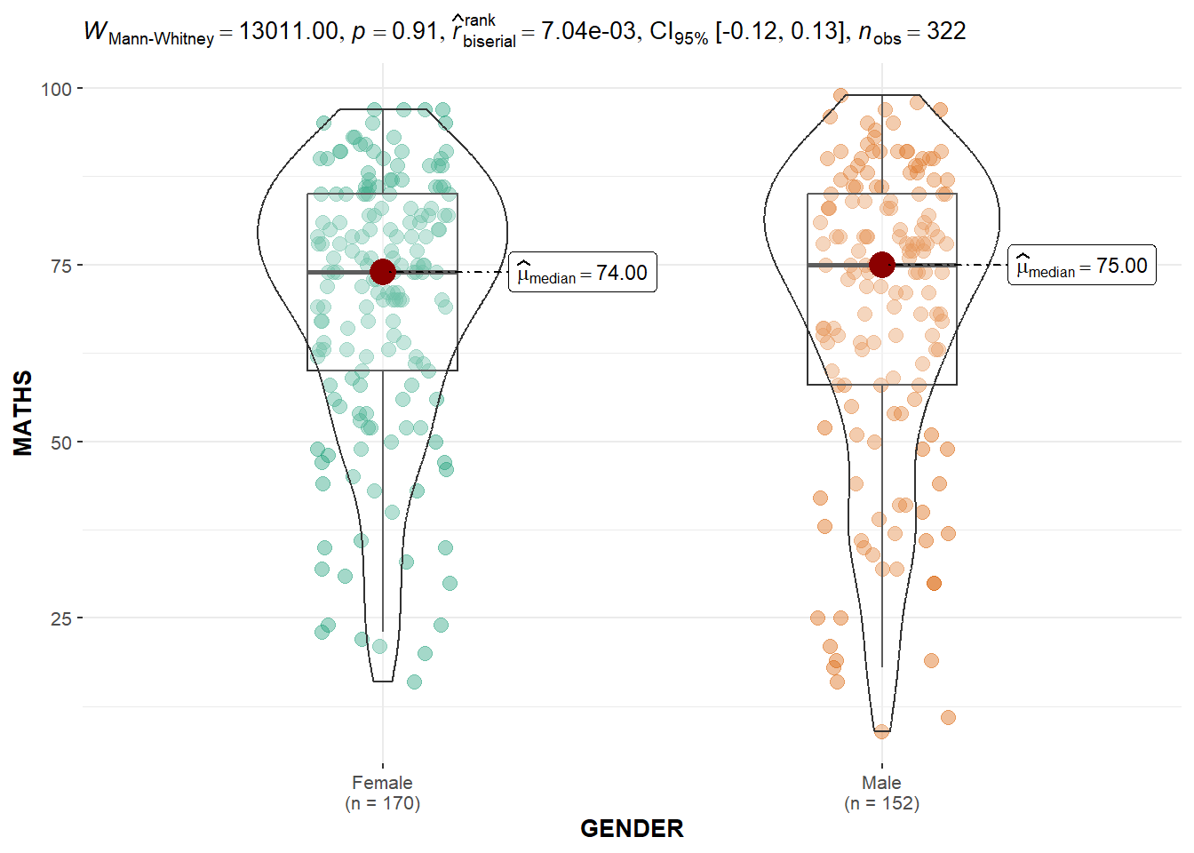
10.3.6 Two-sample mean test: ggbetweenstats()

Two-sample mean test of Maths scores by gender

ggbetweenstats(
  data = exam,
  x = GENDER, 
  y = MATHS,
  type = "np",
  messages = FALSE
)

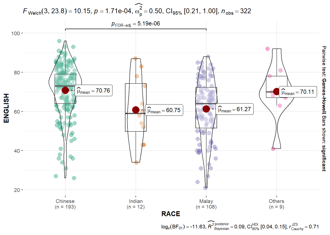
10.3.7 Oneway ANOVA Test: ggbetweenstats() method

• “ns” → only non-significant

• “s” → only significant

• “all” → everything

pairwise.display = “s”

ggbetweenstats(
  data = exam,
  x = RACE, 
  y = ENGLISH,
  type = "p",
  mean.ci = TRUE, 
  pairwise.comparisons = TRUE, 
  pairwise.display = "s",
  p.adjust.method = "fdr",
  messages = FALSE
)

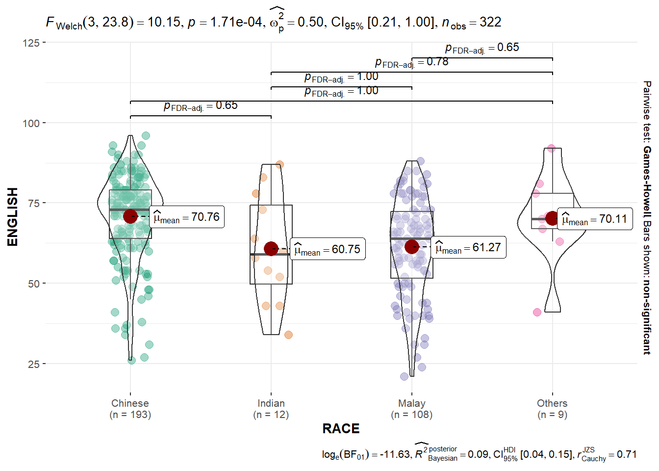
pairwise.display = “ns”

ggbetweenstats(
  data = exam,
  x = RACE, 
  y = ENGLISH,
  type = "p",
  mean.ci = TRUE, 
  pairwise.comparisons = TRUE, 
  pairwise.display = "ns",
  p.adjust.method = "fdr",
  messages = FALSE
)

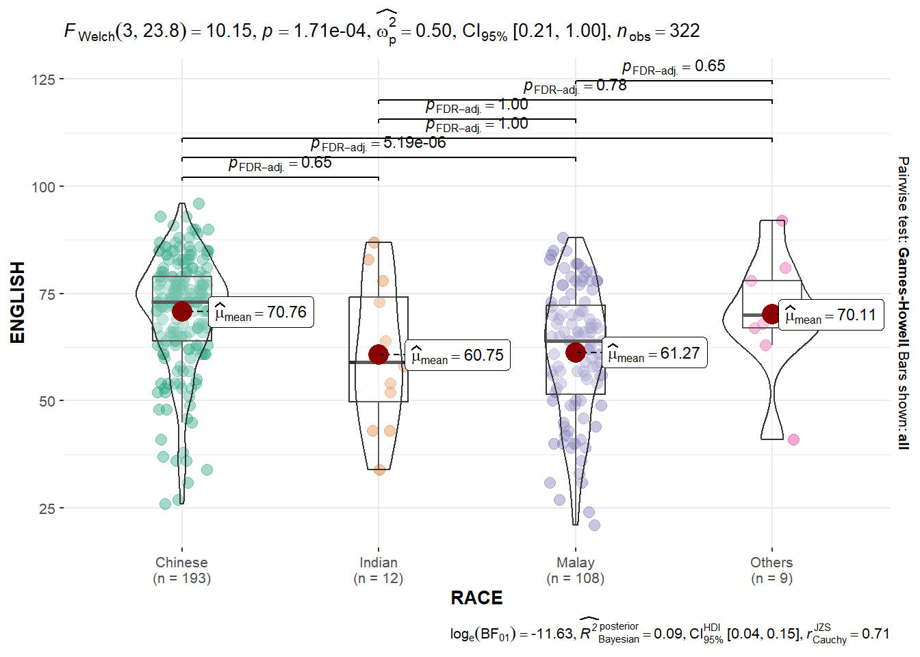
pairwise.display = “all”

ggbetweenstats(
  data = exam,
  x = RACE, 
  y = ENGLISH,
  type = "p",
  mean.ci = TRUE, 
  pairwise.comparisons = TRUE, 
  pairwise.display = "all",
  p.adjust.method = "fdr",
  messages = FALSE
)

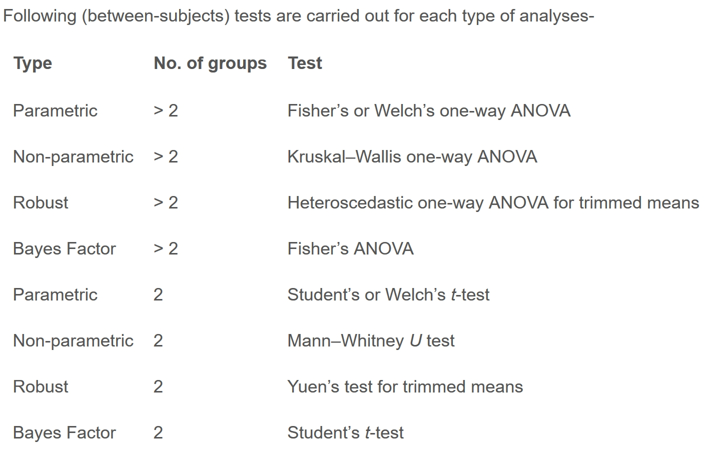
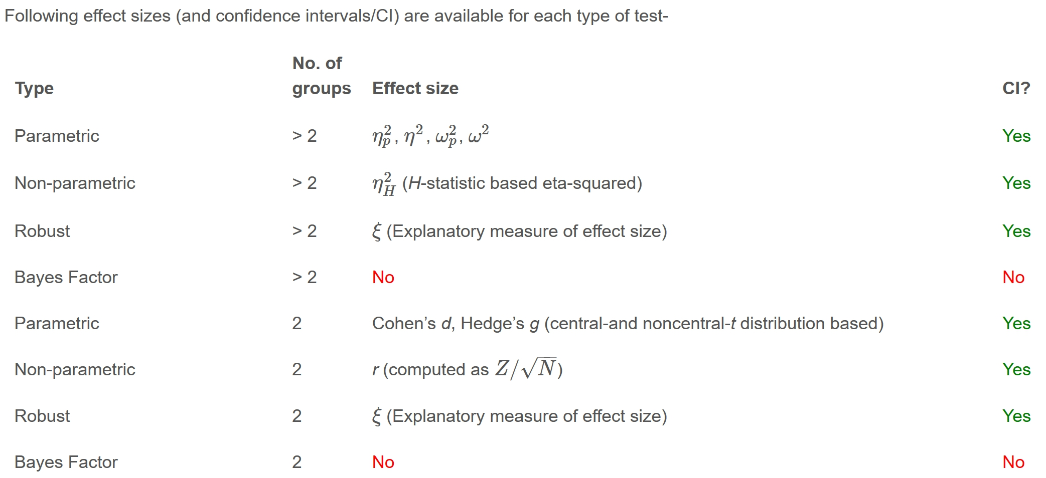
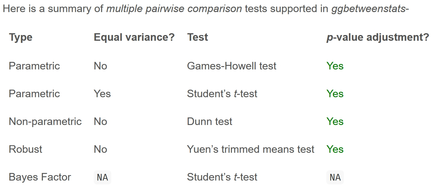
10.3.7.1 ggbetweenstats - Summary of tests

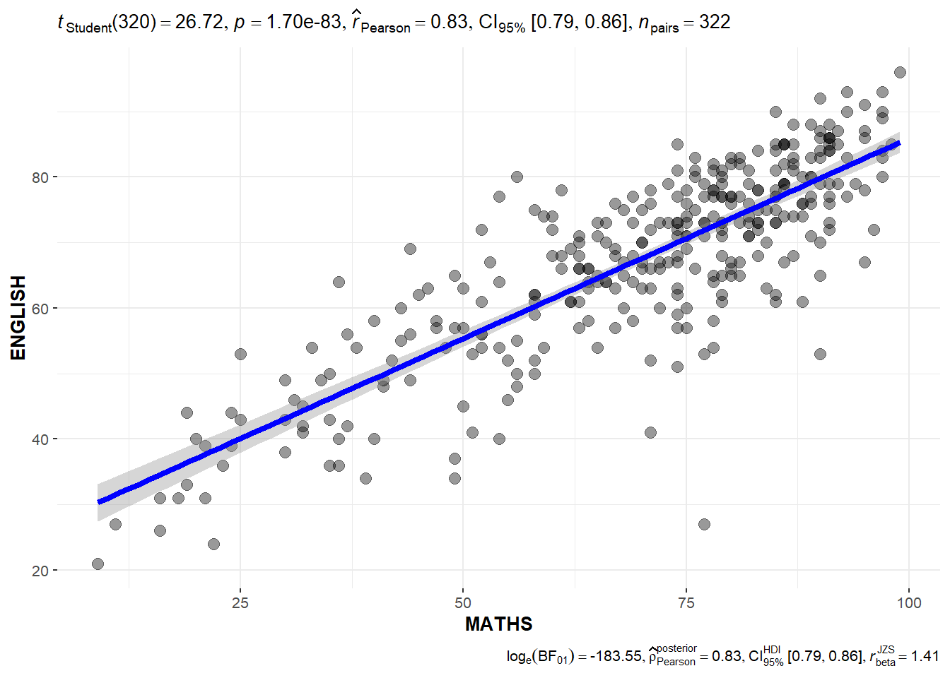
10.3.8 Significant Test of Correlation: ggscatterstats()

ggscatterstats(
  data = exam,
  x = MATHS,
  y = ENGLISH,
  marginal = FALSE,
  )

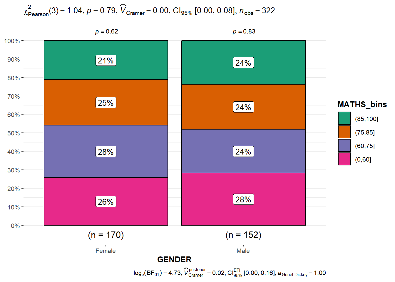
10.3.9 Significant Test of Association (Depedence) : ggbarstats() methods

exam1 <- exam %>% 
  mutate(MATHS_bins = 
           cut(MATHS, 
               breaks = c(0,60,75,85,100))
)

ggbarstats(exam1, 
           x = MATHS_bins, 
           y = GENDER)