pacman::p_load(seriation, dendextend, heatmaply, tidyverse)Hands-on_EX05c
14 Heatmap for Visualising and Analysing Multivariate Data
14.2 Installing and Launching R Packages
14.3 Importing and Preparing The Data Set
14.3.1 Importing the data set
wh <- read_csv("data/WHData-2018.csv")14.3.2 Preparing the data
This command assigns country names as row identifiers in the dataframe, replacing the default numeric row indices.
row.names(wh) <- wh$CountryWarning: Setting row names on a tibble is deprecated.14.3.3 Transforming the data frame into a matrix
The data was loaded into a data frame, but it has to be a data matrix to make your heatmap.
The code chunk below will be used to transform wh data frame into a data matrix.
wh1 <- dplyr::select(wh, c(3, 7:12))
wh_matrix <- data.matrix(wh)
14.4 Static Heatmap
heatmap()of R stats package. It draws a simple heatmap.
heatmap.2() of gplots R package. It draws an enhanced heatmap compared to the R base function.
pheatmap() of pheatmap R package. pheatmap package also known as Pretty Heatmap. The package provides functions to draws pretty heatmaps and provides more control to change the appearance of heatmaps.
ComplexHeatmap package of R/Bioconductor package. The package draws, annotates and arranges complex heatmaps (very useful for genomic data analysis). The full reference guide of the package is available here.
superheat package: A Graphical Tool for Exploring Complex Datasets Using Heatmaps. A system for generating extendable and customizable heatmaps for exploring complex datasets, including big data and data with multiple data types. The full reference guide of the package is available here.
14.4.1 heatmap() of R Stats
- By default, heatmap() plots a cluster heatmap. The arguments Rowv=NA and Colv=NA are used to switch off the option of plotting the row and column dendrograms.
wh_heatmap <- heatmap(wh_matrix,
                      Rowv=NA, Colv=NA)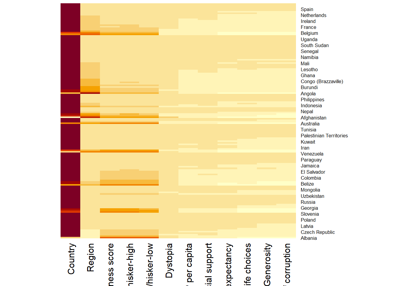
wh_heatmap <- heatmap(wh_matrix)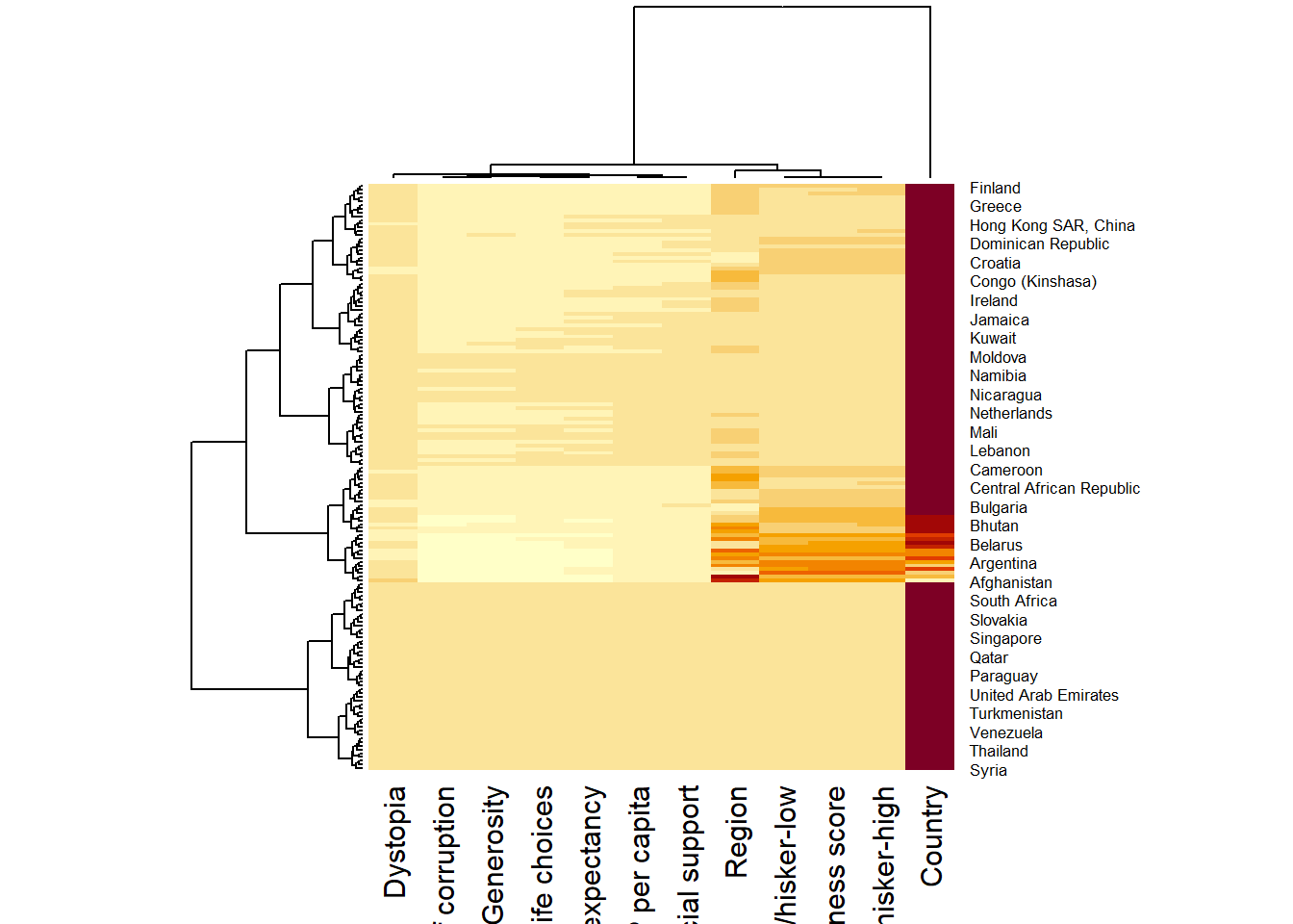
Red cells denotes small values, and red small ones. The Happiness Score variable have relatively higher values, what makes that the other variables with small values all look the same.
Thus, we need to normalize this matrix. This is done using the scale argument. It can be applied to rows or to columns.
wh_heatmap <- heatmap(wh_matrix,
                      scale="column",
                      cexRow = 0.6,
                      cexCol = 0.8,
                      margins = c(10, 4))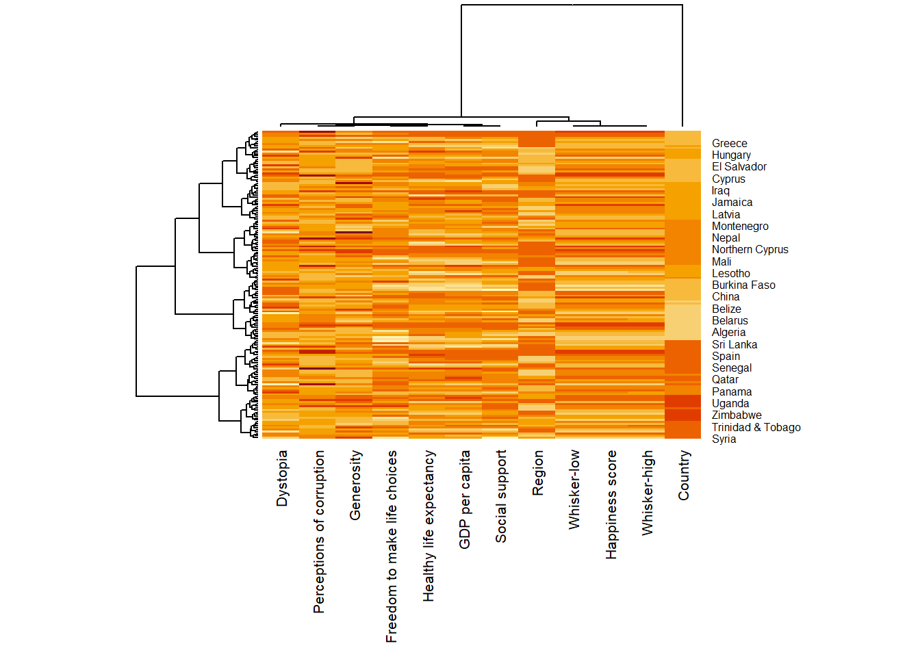
14.5 Creating Interactive Heatmap
14.5.1 Working with heatmaply
heatmaply(mtcars)heatmaply(wh_matrix[, -c(1, 2, 4, 5)])14.5.2 Data trasformation
14.5.2.1 Scaling method
When all variables are came from or assumed to come from some normal distribution, then scaling (i.e.: subtract the mean and divide by the standard deviation) would bring them all close to the standard normal distribution.
heatmaply(wh_matrix[, -c(1, 2, 4, 5)],
          scale = "column")
14.5.2.2 Normalising method
When variables in the data comes from possibly different (and non-normal) distributions.
heatmaply(normalize(wh_matrix[, -c(1, 2, 4, 5)]))14.5.2.3 Percentising method
This is similar to ranking the variables, but instead of keeping the rank values, divide them by the maximal rank.
This is done by using the ecdf of the variables on their own values, bringing each value to its empirical percentile.
The benefit of the percentize function is that each value has a relatively clear interpretation, it is the percent of observations that got that value or below it.
heatmaply(percentize(wh_matrix[, -c(1, 2, 4, 5)]))14.5.3 Clustering algorithm
heatmaply supports a variety of hierarchical clustering algorithm. The main arguments provided are:
distfun: function used to compute the distance (dissimilarity) between both rows and columns. Defaults to dist. The options “pearson”, “spearman” and “kendall” can be used to use correlation-based clustering, which uses as.dist(1 - cor(t(x))) as the distance metric (using the specified correlation method).
hclustfun: function used to compute the hierarchical clustering when Rowv or Colv are not dendrograms. Defaults to hclust.
dist_method default is NULL, which results in “euclidean” to be used. It can accept alternative character strings indicating the method to be passed to distfun. By default distfun is “dist”” hence this can be one of “euclidean”, “maximum”, “manhattan”, “canberra”, “binary” or “minkowski”.
hclust_method default is NULL, which results in “complete” method to be used. It can accept alternative character strings indicating the method to be passed to hclustfun. By default hclustfun is hclust hence this can be one of “ward.D”, “ward.D2”, “single”, “complete”, “average” (= UPGMA), “mcquitty” (= WPGMA), “median” (= WPGMC) or “centroid” (= UPGMC).
In general, a clustering model can be calibrated either manually or statistically.
14.5.4 Manual approach
heatmaply(normalize(wh_matrix[, -c(1, 2, 4, 5)]),
          dist_method = "euclidean",
          hclust_method = "ward.D")
14.5.5 Statistical approach
First, the dend_expend() will be used to determine the recommended clustering method to be used.
We select the higher optimum value.
wh_d <- dist(normalize(wh_matrix[, -c(1, 2, 4, 5)]), method = "euclidean")
dend_expend(wh_d)[[3]]
dist_methods hclust_methods optim
1 unknown ward.D 0.6137851
2 unknown ward.D2 0.6289186
3 unknown single 0.4774362
4 unknown complete 0.6434009
5 unknown average 0.6701688
6 unknown mcquitty 0.5020102
7 unknown median 0.5901833
8 unknown centroid 0.6338734Figure below shows that k=3 would be good.
wh_clust <- hclust(wh_d, method = "average")
num_k <- find_k(wh_clust)
plot(num_k)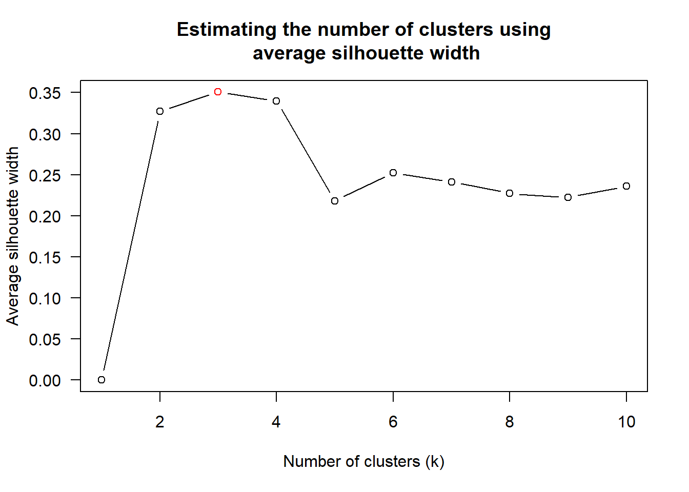
heatmaply(normalize(wh_matrix[, -c(1, 2, 4, 5)]),
          dist_method = "euclidean",
          hclust_method = "average",
          k_row = 3)
14.5.6 Seriation
Optimal Leaf Ordering (OLO). This algorithm starts with the output of an agglomerative clustering algorithm and produces a unique ordering, one that flips the various branches of the dendrogram around so as to minimize the sum of dissimilarities between adjacent leaves. Here is the result of applying Optimal Leaf Ordering to the same clustering result as the heatmap above.
heatmaply(normalize(wh_matrix[, -c(1, 2, 4, 5)]),
          seriate = "OLO")
Another option is “GW” (Gruvaeus and Wainer) which aims for the same goal but uses a potentially faster heuristic.
heatmaply(normalize(wh_matrix[, -c(1, 2, 4, 5)]),
          seriate = "GW")
Registered S3 method overwritten by 'gclus':
method from
reorder.hclust seriationThe option “mean” gives the output we would get by default from heatmap functions in other packages such as gplots::heatmap.2.
heatmaply(normalize(wh_matrix[, -c(1, 2, 4, 5)]),
seriate = "mean")heatmaply(normalize(wh_matrix[, -c(1, 2, 4, 5)]),
seriate = "none")14.5.7 Working with colour palettes
The default colour palette uses by heatmaply is viridis. heatmaply users, however, can use other colour palettes in order to improve the aestheticness and visual friendliness of the heatmap.
heatmaply(normalize(wh_matrix[, -c(1, 2, 4, 5)]),
          seriate = "none",
          colors = Blues)
14.5.8 The finishing touch
In the code chunk below the following arguments are used:
k_row is used to produce 5 groups.
margins is used to change the top margin to 60 and row margin to 200.
fontsizw_row and fontsize_col are used to change the font size for row and column labels to 4.
main is used to write the main title of the plot.
xlab and ylab are used to write the x-axis and y-axis labels respectively.
heatmaply(normalize(wh_matrix[, -c(1, 2, 4, 5)]),
          Colv=NA,
          seriate = "none",
          colors = Blues,
          k_row = 5,
          margins = c(NA,200,60,NA),
          fontsize_row = 4,
          fontsize_col = 5,
          main="World Happiness Score and Variables by Country, 2018 \nDataTransformation using Normalise Method",
          xlab = "World Happiness Indicators",
          ylab = "World Countries"
          )